Linear MHD Workflow
1. Running LMHD Programs from ElVis
The Linear MHD workflow is
integrated with ElVis. The user interface enables you to:
To start a work session, run ElVis and go to: Desktop --> Linear MHD...
2. Data Sources
The data sources consist of EFIT01 from NSTX, Plasma State files, or a TRANSP run.
2.1 EFIT
In the Data Source panel go to the Shot tab to specify source data from EFIT. Enter the NSTX shot number and click on Get Times. This will return a list of times when EFIT has been run. Click on a time to use and click Retrieve. This will get a Plasma State file for the specified time and display 4 graphs. The entire Plasma State is in the graph window so additional plots can be constructed. The data is store in the run directory shown as Next Run ID. Text output from the retrieval is shown in the Status panel. The Pest program works with 1 or more EFIT times as the source data. All other codes work with source data from just 1 EFIT time.
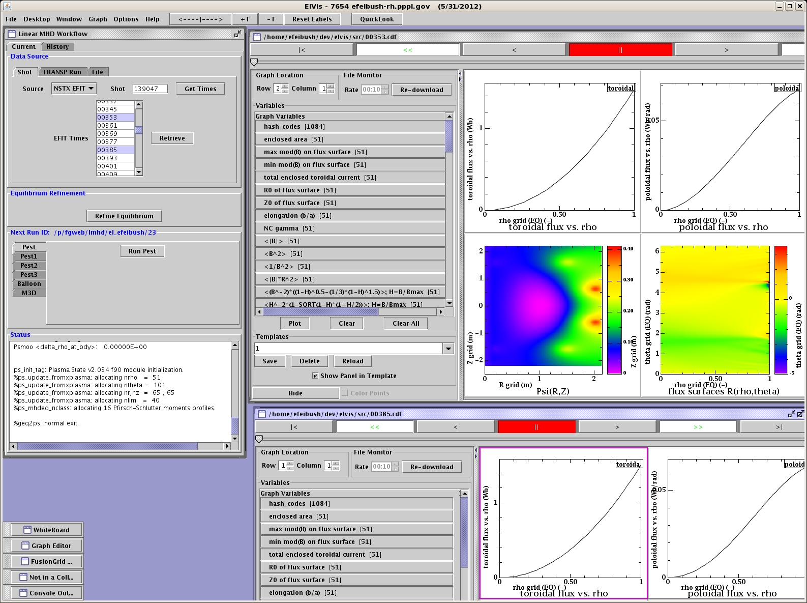
Figure 1 - Retrieve source data from available EFIT times. Time indices 353 and 385 have been selected for a Pest run. All other programs start with just 1 time index.
2.2 TRANSP Run
In the Data Source panel go to the TRANSP Run tab. Enter the Run ID, time of interest, and time average. Click on Retrieve to extract a plasma state for the specified time. A graph window is displayed with 6 graphs. The entire plasma state is in the window so additional plots can be constructed.
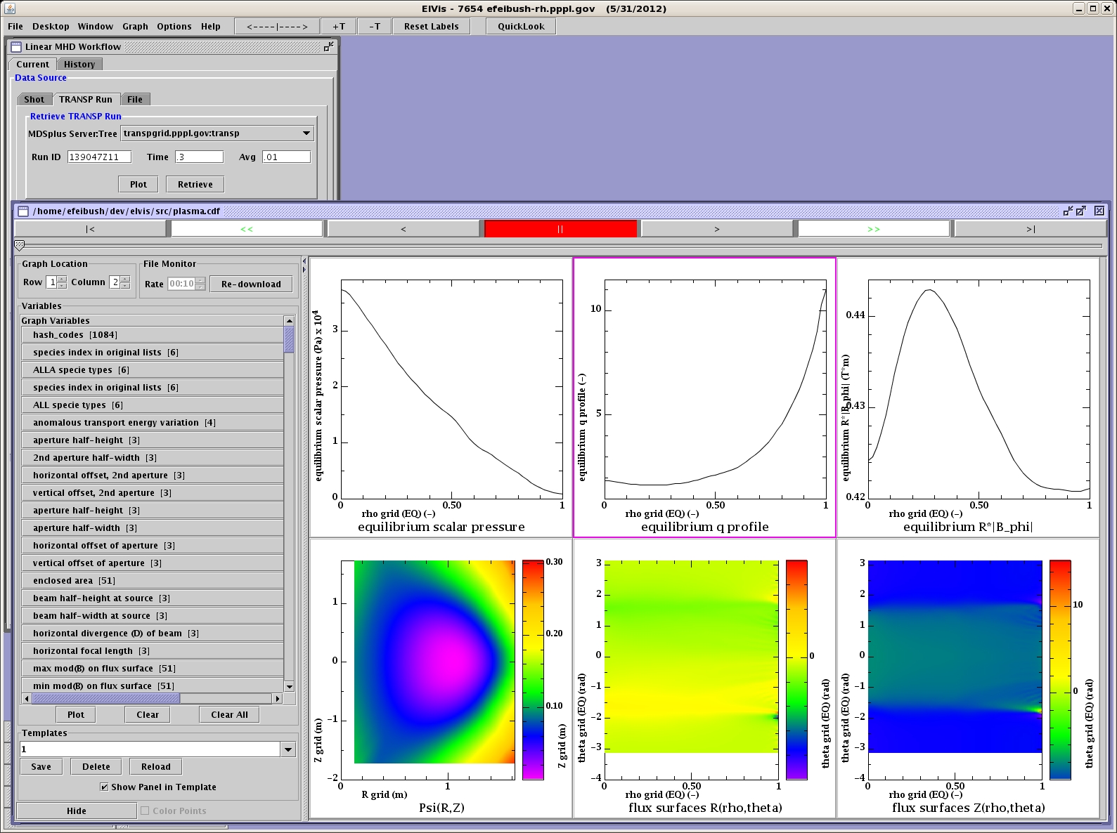
Figure 2 - Retrieve source data from a TRANSP run.
The data for the TRANSP run can be examined in RPLOT within ElVis by clicking on Plot. This will bring up an RPLOT session within ElVis. You can enter RPLOT commands or scripts to plot graphs from the run.
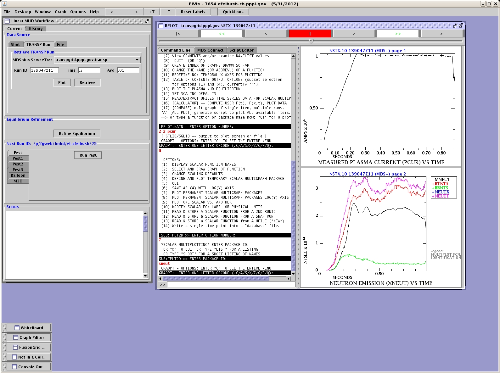
Figure 3 - Running RPLOT within ElVis to examine data from a TRANSP run.
2.3 Importing Files
Existing files can be imported as the source to an LMHD run. Select the type of file to import as either GEQ file, Plasma State file, EQDSKA file, or a Refined Equilibrium (eqb1) file. Enter the name of the file in the text field and click Import.
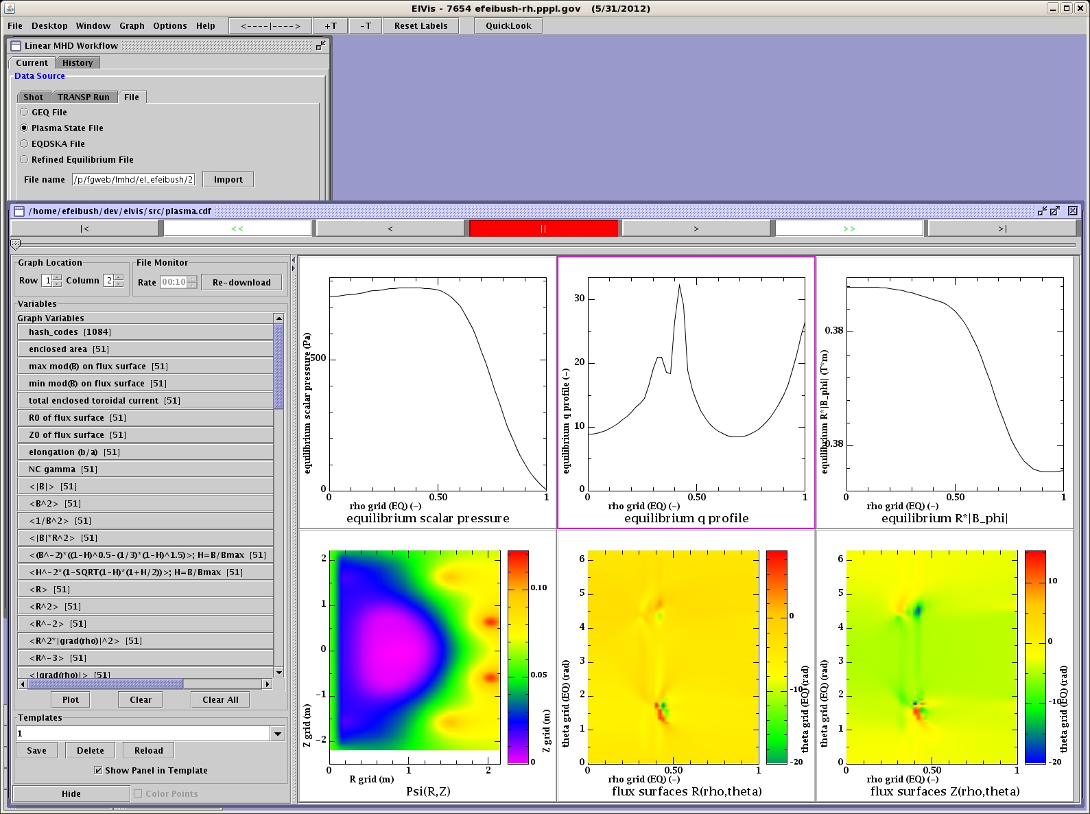
Figure 4 - Importing a Plasma State file.
3. Equilibrium Refinement
The LMHD programs work from a refined equilibrium. The workflow will run JSolver to produce an eqb1 file and an eqdsk.cdf file in the run directory. Click on Refine Equilibrium to run JSolver. Two graphs from the resulting plasma state will be displayed and the text output will be shown in the Status panel.
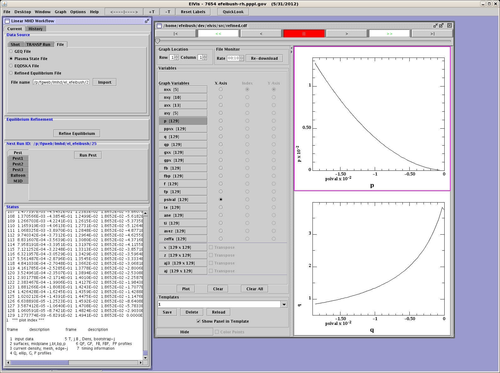
Figure 5 - Equilibrium refinement computed by JSolver.
4. LMHD Programs
An LMHD program can be run after the equilibrium refinement stage. Select the program by clicking on one of the tabs along the left edge of the Run panel. Then click the Run button. M3D has 4 additional menus. The Sim tab contains the name list where the value of each parameter can be set for M3D-C1. The PETSC tab has the name list for the PETSC portion of the simulation. The CPUs tab lets you control the number of cpus assigned to the run. The Job tab has fields for setting the maximum amount of CPU time and selecting the batch queue where the job will be run on hopper at Nersc. Click the Run M3D button to submit a job. You must have an account at Nersc and a batch allocation in order to run M3D-C1.
1. Select a data source,
retrieve, and display data.
2. Refine the equilibrium.
3. Run an LMHD program, such as Pest, Pest1, Pest2, Pest3, Balloon, or M3D-C1.
4. Display results from different runs.
5. Manage runs through the Run History table.
1.1 The LMHD Workflow2. Refine the equilibrium.
3. Run an LMHD program, such as Pest, Pest1, Pest2, Pest3, Balloon, or M3D-C1.
4. Display results from different runs.
5. Manage runs through the Run History table.
To start a work session, run ElVis and go to: Desktop --> Linear MHD...
2. Data Sources
The data sources consist of EFIT01 from NSTX, Plasma State files, or a TRANSP run.
2.1 EFIT
In the Data Source panel go to the Shot tab to specify source data from EFIT. Enter the NSTX shot number and click on Get Times. This will return a list of times when EFIT has been run. Click on a time to use and click Retrieve. This will get a Plasma State file for the specified time and display 4 graphs. The entire Plasma State is in the graph window so additional plots can be constructed. The data is store in the run directory shown as Next Run ID. Text output from the retrieval is shown in the Status panel. The Pest program works with 1 or more EFIT times as the source data. All other codes work with source data from just 1 EFIT time.
Figure 1 - Retrieve source data from available EFIT times. Time indices 353 and 385 have been selected for a Pest run. All other programs start with just 1 time index.
2.2 TRANSP Run
In the Data Source panel go to the TRANSP Run tab. Enter the Run ID, time of interest, and time average. Click on Retrieve to extract a plasma state for the specified time. A graph window is displayed with 6 graphs. The entire plasma state is in the window so additional plots can be constructed.
Figure 2 - Retrieve source data from a TRANSP run.
The data for the TRANSP run can be examined in RPLOT within ElVis by clicking on Plot. This will bring up an RPLOT session within ElVis. You can enter RPLOT commands or scripts to plot graphs from the run.
Figure 3 - Running RPLOT within ElVis to examine data from a TRANSP run.
2.3 Importing Files
Existing files can be imported as the source to an LMHD run. Select the type of file to import as either GEQ file, Plasma State file, EQDSKA file, or a Refined Equilibrium (eqb1) file. Enter the name of the file in the text field and click Import.
Figure 4 - Importing a Plasma State file.
3. Equilibrium Refinement
The LMHD programs work from a refined equilibrium. The workflow will run JSolver to produce an eqb1 file and an eqdsk.cdf file in the run directory. Click on Refine Equilibrium to run JSolver. Two graphs from the resulting plasma state will be displayed and the text output will be shown in the Status panel.
Figure 5 - Equilibrium refinement computed by JSolver.
4. LMHD Programs
An LMHD program can be run after the equilibrium refinement stage. Select the program by clicking on one of the tabs along the left edge of the Run panel. Then click the Run button. M3D has 4 additional menus. The Sim tab contains the name list where the value of each parameter can be set for M3D-C1. The PETSC tab has the name list for the PETSC portion of the simulation. The CPUs tab lets you control the number of cpus assigned to the run. The Job tab has fields for setting the maximum amount of CPU time and selecting the batch queue where the job will be run on hopper at Nersc. Click the Run M3D button to submit a job. You must have an account at Nersc and a batch allocation in order to run M3D-C1.