Example 3 - vector plots

Example 3 - vector plots |
|
To run this example, you must download the following files:
gsun03n.ncland then type:
gsn_code.ncl
ncl < gsun03n.ncl
| Frame 1 | Frame 2 | Frame 3 | Frame 4 |
|---|---|---|---|
| 
| 
| 
|
(Click on any frame to see it enlarged.)
  1. load "gsn_code.ncl"
  2.
  3. begin
  4.   dir = ncargpath("data")
  5.   uf = addfile(dir+"/cdf/Ustorm.cdf","r")  ; Open two netCDF files.
  6.   vf = addfile(dir+"/cdf/Vstorm.cdf","r")
  7.
  8.   u   = uf->u(0,:,:)   ; Get u, v, latitude, and longitude data.
  9.   v   = vf->v(0,:,:)
 10.   lat = uf->u&lat
 11.   lon = uf->u&lon
 12.
 13.   wks = gsn_open_wks("x11","gsun03n") ; Open a workstation.
 14.
 15.   vc = gsn_vector(wks,u,v,False)    ; Draw a vector plot of u and v.
 16.
 17. ;----------- Begin second plot -----------------------------------------
 18.
 19.   resources = True
 20.
 21.   resources@vcMinFracLengthF = 0.33
 22.   resources@vcRefMagnitudeF  = 20.0
 23.   resources@vcRefLengthF     = 0.045
 24.
 25.   resources@vcMonoLineArrowColor  = False   ; Draw vectors in color.
 26.
 27.   vc = gsn_vector(wks,u,v,resources)
 28.
 29. ;----------- Begin third plot -----------------------------------------
 30.
 31.   resources@tiMainString  = ":F26:wind velocity vectors - January 1996"
 32.   resources@tiXAxisString = "longitude"
 33.   resources@tiYAxisString = "latitude"
 34.
 35.   resources@vfXCStartV  = lon(0)               ; Define X/Y axes range
 36.   resources@vfXCEndV    = lon(dimsizes(lon)-1) ; for vector plot.
 37.   resources@vfYCStartV  = lat(0)
 38.   resources@vfYCEndV    = lat(dimsizes(lat)-1)
 39.
 40.   resources@pmLabelBarDisplayMode    = "Always"   ; Turn on a label bar.
 41.   resources@pmLabelBarWidthF         = 0.1
 42.   resources@lbPerimOn                = False
 43.
 44.   vc = gsn_vector(wks,u,v,resources)
 45.
 46. ;---------- Begin fourth plot ------------------------------------------
 47.
 48.   tf = addfile(dir+"/cdf/Tstorm.cdf","r")    ; Open a netCDF file.
 49.   temp  = (tf->t(0,:,:)-273.15)*9.0/5.0+32.0 ; Read in temp data and
 50.                                              ; convert from K to F.
 51.   temp@units = "(deg F)"
 52.
 53.   cmap = (/(/1.00, 1.00, 1.00/), (/0.00, 0.00, 0.00/), \
 54.            (/.560, .500, .700/), (/.300, .300, .700/), \
 55.            (/.100, .100, .700/), (/.000, .100, .700/), \
 56.            (/.000, .300, .700/), (/.000, .500, .500/), \
 57.            (/.000, .700, .100/), (/.060, .680, .000/), \
 58.            (/.550, .550, .000/), (/.570, .420, .000/), \
 59.            (/.700, .285, .000/), (/.700, .180, .000/), \
 60.            (/.870, .050, .000/), (/1.00, .000, .000/), \
 61.            (/.700, .700, .700/)/)
 62.
 63.   gsn_define_colormap(wks, cmap)  ; Define a new color map.
 64.
 65.   resources@vcFillArrowsOn           = True  ; Fill the vector arrows
 66.   resources@vcMonoFillArrowFillColor = False ; in different colors
 67.   resources@vcFillArrowEdgeColor     = 1     ; Draw the edges in black.
 68.   resources@vcFillArrowWidthF        = 0.055 ; Make vectors thinner.
 69.
 70.   resources@tiMainString      = ":F26:wind velocity vectors colored by temperature " + temp@units
 71.   resources@tiMainFontHeightF = 0.02  ; Make font slightly smaller.
 72.   resources@lbLabelFont       = 21    ; Change font of label bar labels.
 73.
 74.   vc = gsn_vector_scalar(wks,u,v,temp,resources) ; Draw a vector plot of
 75.                                                  ; u and v and color them
 76.                                                  ; according to the scalar
 77.                                                  ; field "temp."
 78.   delete(vc)    ; Clean up.
 79.   delete(u)
 80.   delete(v)
 81.   delete(temp)
 82. end
load "gsn_code.ncl"
Load the NCL script that contains the functions and procedures (the ones that start with "gsn_") that are used in this example. load in NCL works much like include works in C and Fortran 90 programs.
begin
Begin the NCL script.
dir = ncargpath("data")
The function ncargpath
returns the absolute pathname of the NCAR Graphics directory name that
is passed to it. The directory "data" is a directory containing
sample netCDF, GRIB, ASCII, and binary files for use by these examples
and other NCAR Graphics examples.
  uf = addfile(dir+"/cdf/Ustorm.cdf","r")
  vf = addfile(dir+"/cdf/Vstorm.cdf","r")
Open two netCDF files containing wind velocity vector data with addfile. The addfile function is described in example 2.
  u   = uf->u(0,:,:)
  v   = vf->v(0,:,:)
  lat = uf->u&lat
  lon = uf->u&lon
Read the variables u and v and the coordinate variables lat and lon from two of the netCDF file references, uf and vf and store them to local NCL variables.
uf->u and vf->v are 3-dimensional arrays (of the same size) of wind velocity vector data, where the first dimension represents time steps, the second dimension represents the latitude values that the vector field is measured on, and the third dimension represents the longitude values of the vector field. By using the syntax (0,:,:), you are selecting the vector field for the full latitude/longitude range for the first time step only.
uf->u&lat and uf->v&lon are 1-dimensional coordinate variables of u and v, so they give the actual latitude and longitude ranges that the vector field is measured on. By definition of a coordinate variable, uf->u&lat has the same dimension as the second dimension of uf->u and vf->v, and uf->u&lon has the same dimension as the third dimension of uf->u and vf->v.
wks = gsn_open_wks("x11","gsun03n")
Open an X11 workstation for which to draw the vector plots.
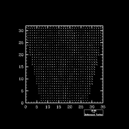
vc = gsn_vector(wks,u,v,False)Create and draw a vector plot of the 2-dimensional arrays u and v. The first argument of the gsn_vector function is the workstation variable returned from the previous call to gsn_open_wks. The next two arguments represent the 2-dimensional vector field to be vectorized (they must have the same dimensions and can be of type float, double, or integer). The last argument is a logical value indicating whether you have set any resources. To get the default vector plot that NCL provides, pass the value False for the last argument.
The default vector plot drawn contains labeled tick marks and a "reference vector" label at the bottom right of the plot. Since no ranges have been defined for the X and Y axes in this plot, the range values default to 0 to n-1, where n is the number of points in that dimension. By default, vectors are drawn with lines and hollow arrow heads, but you can change them to filled vectors as you'll see in a later frame in this example.
Note that there are some areas in the vector plot where no vectors are drawn. This is due to the presence of missing values in the data. By default, if the data being passed to any of the gsn_* plotting routines contains the attribute "_FillValue," then the value of this attribute is assumed to represent a missing value, and the gsn_* routines do not plot any data equal to this value.
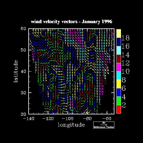
;----------- Begin second plot -----------------------------------------Draw the same vector plot, only this time set some resources to change the length of the vectors and draw them in color.
resources = TrueGet ready to set up a list of resources for changing the look of the plot. See example 1 for an explanation of how resources are set. Vector plot resources are part of the "VectorPlot" group and all start with the letters "vc". They are documented in the "VectorPlot resource descriptions" section of the NCAR Graphics 4.1 Reference Manual.
Data associated with a vector plot is called a "VectorField." VectorField resources start with "vf" and are documented in the "VectorField resource descriptions" section of the NCAR Graphics 4.1 Reference Manual.
resources@vcMinFracLengthF = 0.33The vcMinFracLengthF resource sets the length of the minimum magnitude vector as a fraction of the length of the reference vector (the default is 0).
  resources@vcRefMagnitudeF  = 20.0
  resources@vcRefLengthF     = 0.045
The vcRefMagnitudeF resource indicates which magnitude to use for the reference magnitude (the default is 0, a special value that indicates that the maximum magnitude in the vector field is used as a reference magnitude). vcRefLengthF sets the length of the reference magnitude in NDC coordinates (this resource is normally set dynamically according to the number of elements in the vector field and the size of the plot's viewport).
resources@vcMonoLineArrowColor = FalseTo draw vectors in color, set vcMonoLineArrowColor to False, indicating that you don't want all of the vectors drawn in a single color. The default color table is used, and it can be seen in the "color tables" section of the NCAR Graphics 4.1 Reference Manual.
vc = gsn_vector(wks,u,v,resources)Draw the new vector plot using the resources you just set.
;----------- Begin third plot -----------------------------------------Draw the same vector plot, only set some resources to change the the X and Y axis ranges, and add a label bar and a title.
  resources@tiMainString  = ":F26:wind velocity vectors - January 1996"
  resources@tiXAxisString = "longitude"
  resources@tiYAxisString = "latitude"
Create a title and labels for the X and Y axes. NCL allows special text functions to be embedded in strings to indicate you want things like sub/superscripting, different fonts, carriage returns, etc. By default, each special function is preceded and succeeded with a colon. In the string for the tiMainString resource, the ":F26:" part is a text function indicating that you want to use font 26, which is Times-bold.
If you happen to have a colon as part of the string, and you don't want it to be interpreted as a function code, then you can use the txFuncCode resource to change the function code character. The various text function codes are documented in the "Text function codes" section of the NCAR Graphics 4.1 Reference Manual.
  resources@vfXCStartV  = lon(0)
  resources@vfXCEndV    = lon(dimsizes(lon)-1)
  resources@vfYCStartV  = lat(0)
  resources@vfYCEndV    = lat(dimsizes(lat)-1)
The resources vfXCStartV and vfXCEndV indicate the starting and ending data locations along the X axis of the vector field you are plotting. Likewise, vfYCStartV and vfYCEndV indicate the starting and ending data locations along the Y axis of the vector field. If you don't set these resources, then the vf*StartV resources default to 0.0 and the vf*EndV resources default to the number of data elements in that direction minus 1.
The function dimsizes returns the dimension sizes of the variable passed to it. In this case, lat and lon are 1-dimensional arrays, so dimsizes returns the length of each array.
  resources@pmLabelBarDisplayMode    = "Always"
  resources@pmLabelBarWidthF         = 0.1
  resources@lbPerimOn                = False
Turn on the drawing of a label bar, change its width, and turn off its perimeter. A discussion on the "pm" (PlotManager) resources appears in example 2.
vc = gsn_vector(wks,u,v,resources)Draw the third vector plot with the new resources that you added.
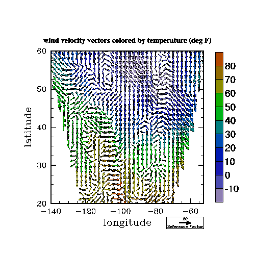
;---------- Begin fourth plot ------------------------------------------Create your own color map, color the vectors according to a separate temperature scalar field, and fill the vector arrows.
  tf = addfile(dir+"/cdf/Tstorm.cdf","r")
  temp  = (tf->t(0,:,:)-273.15)*9.0/5.0+32.0

  temp@units = "(deg F)"
Open a netCDF file containing temperature data, read in the first level of the temperature data and convert it from Kelvin to Fahrenheit, and update the "units" attribute. The temperature data is measured over the same time steps and latitude/longitude grid as the wind velocity vector data that you read in earlier.
  cmap = (/(/1.00, 1.00, 1.00/), (/0.00, 0.00, 0.00/), \
           (/.560, .500, .700/), (/.300, .300, .700/), \
           (/.100, .100, .700/), (/.000, .100, .700/), \
           (/.000, .300, .700/), (/.000, .500, .500/), \
           (/.000, .700, .100/), (/.060, .680, .000/), \
           (/.550, .550, .000/), (/.570, .420, .000/), \
           (/.700, .285, .000/), (/.700, .180, .000/), \
           (/.870, .050, .000/), (/1.00, .000, .000/), \
           (/.700, .700, .700/)/)

  gsn_define_colormap(wks, cmap)
Define your own color map. Details on creating your own color map are
covered in example 2.
  resources@vcFillArrowsOn           = True
  resources@vcMonoFillArrowFillColor = False
  resources@vcFillArrowEdgeColor     = 1
  resources@vcFillArrowWidthF        = 0.055
Setting the vcFillArrowsOn resource to True produces filled vector arrows instead of vector arrows drawn with lines. Setting vcMonoFillArrowFillColor to False fills the vector arrows using multiple colors.
By default, the vcFillArrowEdgeColor resource is set to the background color (index 0). By changing this to the foreground color (index 1), you are making the vector arrows more visible. The vcFillArrowWidthF resource sets the width of the arrows as a fraction of the vcRefLengthF. The default is 0.1.
There's a handy vector arrow diagram in the description of VectorPlot that shows the various components of a vector arrow.
  resources@tiMainString      = ":F26:wind velocity vectors colored by temperature " + temp@units
  resources@tiMainFontHeightF = 0.02
  resources@lbLabelFont       = 21
Change the title for the plot and decrease the size of the font. Also, change the font of the title to 26 (Times-bold) and the font of the label bar labels to 21 (Helvetica). Remember: predefined strings, like those listed in the font table, are case-insensitive, and you could have specified the above fonts with "times-roman" or "HELVETICA" or any another combination of uppercase and lowercase characters.
vc = gsn_vector_scalar(wks,u,v,temp,resources)Use the gsn_vector_scalar function to draw a vector plot and color the vectors according to the scalar field temp. The gsn_vector_scalar function is the same as the gsn_vector function, only it has a scalar field as an additional argument (the fourth argument). The scalar field must have the same dimensions as the U and V arrays.
  delete(vc)
  delete(u)
  delete(v)
  delete(temp)
Clean up by deleting some variables you don't need any more.
end
End the NCL script.