4.4 Slice objects

A Slice object is created by taking a slice through a Mesh3d object or perhaps an earlier-created Slice. There are two types of Mesh3d Slices: an isosurface slice (i. e., a surface where some specified function on the Mesh3d has a constant value), and a plane slice (as created by slicing with a Plane object). A pre-existing Slice can be sliced only by a Plane, and the user has the option of retaining both slices, or of discarding one or the other (useful for seeing inside closed isosurfaces, for example).

The user will not normally instantiate a Slice directly, but rather, by invoking the sslice function, which does all the work and returns the resulting Slice.

Creation of a Slice

Isosurface Slice

from mesh3d import *

sl = sslice (m, val [, varno])

The arguments are as follows:

m: a Mesh3d object to be sliced.

val: the value of the function on the isosurface.

varno: the number of the variable for the isosurface; defaults to 1 if not specified. (Recall that the argument c to a Mesh3d can be a vector of values, in which case isosurfaces for several different functions can be plotted on the same graph.)

Upon return from function sslice, sl will be assigned the specified Slice object, or None, if it does not exist.

Plane Slice of Mesh3d

from mesh3d import *

sl = sslice (m, plane [, varno])

The arguments are as follows:

m: a Mesh3d object to be sliced.

plane: a Plane object by which to slice the specified Mesh3d.

varno: the number of the variable used to color the slicing plane; defaults to 1 if not specified. (Recall that the argument c to a Mesh3d can be a vector of values, in which case isosurfaces for several different functions can be plotted on the same graph.)

Upon return from function sslice, sl will be assigned the specified Slice object, or None, if it does not exist.

Plane Slice of a Slice

from mesh3d import *

sl = sslice (s, plane [, nslices])

The arguments are as follows:

s: a Slice object to be sliced.

plane: a Plane object by which to slice the specified Slice:

nslices: if nslices = 1 (the default) then return the piece in front of the Plane; if nslices = 2, return the pair [front, back] of slices. (If you want just the "back" surface, you can achieve this by calling slice with nslices = 1 and - plane instead of plane.)

Upon return from function sslice, sl will be assigned the specified Slice object(s), or None, or [None, None], if it (they) does (do) not exist.

Instantiation

The user will most likely use the sslice function to create Slice objects, rather than instantiating them directly; but here, for the sake of completeness, is direct instantiation.

from mesh3d import *

sl = Slice (nv, xyzv [, val [, plane [, iso]]])

Description

The arguments are as follows:

nv is a one-dimensional integer array whose i^th entry is the number of vertices of the i^th face of the object being sliced.

xyzv is a two-dimensional array dimensioned sum (nv) by 3. The first nv [0] triples in xyzv are the coordinates of the vertices of face [0], the next nv [1] triples are the coordinates of the vertices of face [1], etc.

val (if present) is an array the same length as nv whose i^th entry specifies a color for face i.

plane (if present) says that this is a plane slice, and all the vertices xyzv lie in this plane.

iso (if present) says that this is the isosurface for the given value.

A Slice object or two Slice objects are created by a call to the function sslice (See "Creation of a Slice" on page 70). The function sslice accepts either a mesh and a specification of how to slice it (isosurface or plane), or else a previously created slice, a plane to slice it with, and whether you want to keep the resulting "front" slice or both slices.

Example 1 (a PyGist plot):

This example reads in the same data as the first PyNarcisse example ("Example 1 (a PyNarcisse plot):" on page 66). The data is already in AVS order, so it does not need to be rearranged. This example takes three plane sections through the imploding sphere, and graphs them with color-filled contours and a color bar. The actual plot is shown in Chapter 5, page 97.

from mesh3d import *

from plane import *

from graph3d import *

f = PR ('./bills_plot')

n_nodes = f.NumNodes

n_z = f.NodesOnZones

x = f.XNodeCoords

y = f.YNodeCoords

z = f.ZNodeCoords

c = f.ZNodeVelocity

n_zones = f.NumZones

m1 = Mesh3d (x = x, y = y, z = z, c = c, avs = 1,

hex = [n_zones, n_z])

# Now define the three planes:

pyz = Plane (array ([1., 0., 0.], Float ),

array ( [0.0001, 0., 0.], Float))

pxz = Plane (array ([0., 1., 0.], Float ),

array ( [0., 0.0001, 0.], Float))

p2 = Plane (array ([1., 0., 0.], Float ),

array ( [0.35, 0., 0.], Float))

# Now define the three slices

s2 = sslice (m1, pyz, varno = 1, opt_3d = ["wm", "s4"])

s22 = sslice (m1, p2, varno = 1, opt_3d = ["wm", "s4"])

s23 = sslice (m1, pxz, varno = 1, opt_3d = ["wm", "s4"])

# Create the graph

g1 = Graph3d( [s2, s22, s23], color_card = "rainbow.gp",

opt_3d = ["wm", "s4"], mask = "min", color_bar = 1,

split = 0, hardcopy = "talk.ps")

# plot the graph

g1.plot ()

Example 2 (a PyGist plot):

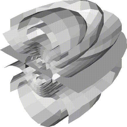
Now we shall plot three isosurfaces of the same sphere shaded by a light source (opt_3d = "none"). The isosurfaces are nested and one will block our view of another, so we slice it for better visibility. Note that the slices isosurface is disconnected, because you see two sliced pieces!

s1 = sslice (m1, .9 * max (c), varno = 1)

s2 = sslice (m1, .9 * min (c), varno = 1, opt_3d = "none")

s5 = sslice (m1, .5 * max (c), varno = 1, opt_3d = "none")

s6 = sslice (s5, -pyz, opt_3d = "none")

g1.set_surface_list ( [s1, s2, s6])

g1.plot ()

Example 3 (a PyGist plot):

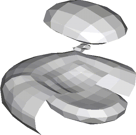
The next plot consists of a number of isosurfaces of the above imploding sphere shaded by a light source (opt_3d = "none"). The isosurfaces are nested and some are closed, so we slice all of them in half and keep the ``back'' halves for visibility.

for i in range (8) :

sl = sslice (m1, .9 * min (c) + i * (.9 * max (c) - .9 *

min (c)) / 8., varno = 1, opt_3d = "none")

slice_list.append (sslice (sl, pxz))

g1.set_surface_list ( slice_list)

g1.plot ()