Python modules for data visualization and postprocessing, as well as python wrappers for IPEC and PENT.
| Author: | N.C. Logan |
|---|---|
| Location: | Princeton Plasma Physics Laboratory |
| Email: | nlogan@pppl.gov |
To set up python on portal at PPPL, insert the following lines into your .bashrc file:
export PYTHONPATH=$PYTHONPATH:/p/gpec/users/nlogan/ipec_3.00/nlogan module load python/2.7.2
For tcsh shell users, replace export with setenv syntax and insert in .cshrc. For gpec owners, replace /p/gpec/users/nlogan/ipec_3.00/nlogan with the top level directory for your own branch of ipec if you have one.
To put the changes into effect:
$ source ~/.bashrc
The 3 workhorse modules for scientific programming in python are numpy, scipy and matplotlib (although the third is really a personal preference). Tutorials for each can be found at
To set personal defualts for runs, edit the _defaults_.py file in this directory. Some of these (like email) should be obvious, others you may not understand until becoming more familiar with the package. Do not worry if these are confusing, and feel free to skip them for now.
The ipython (interactive) environment is recomended for commandline data analysis. To start, it is easiest to auto-import a number of basic mathematic and visualization modules and use an enhanced interactivity for displaying figures. To do this enter:
$ ipython –pylab
Look into online tutorial on numpy and matplotlib. Advanced users are recomended to edit ~/.matplotlib/matplotlibrc and ~/.ipython/profile_default/startup/autoimports.ipy files.
Now in the ipython envirnment, type
>>> from pypec import *
WARNING: Mayavi not in python path
WARNING: USING PORTAL - "use -w 24:00:00 -l mem=8gb" recomended for heavy computation
This will import a number of modules, the most important of which are gpec, and data. There may be a few warnings/hints... ignore them for now.
The data module is a very generalized tool for visualizing and manipulating scientific data from ascii files. The only requirement for creating a data object is that the file have one or more tables of data, with appropriate labels in a header line directly above the data.
Here, we show some examples using common outputs from both IPEC and PENT.
First, in an open ipython session, explore the data module by typing ‘data.’ and hitting tab. For information on any particular object in the module, use the ‘?’ syntax or ‘help’ function. For example, enter ‘data.read?’. You will see that it has a lot of metadata on this function, but the important things to look at for now are the arguments and key word arguments. These are passed to the function as shown in the Definition line... you can either pass a single string, or a string and specification for squeeze. If this confuses you, consult any of the many great python tutorials online.
Lets use it! To read an ascii file containing tablular data use the read function.
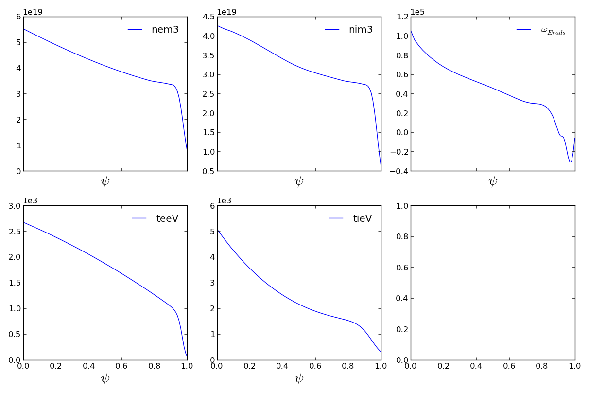
>>> mydata = read('examples/example_profiles.dat')
Casting table 1 into Data object.
>>> type(mydata),len(mydata)
(<type 'list'>, 1)
The read function creates a list of data objects corresponding to the tables in the text file. In this case, there is only one table. If we knew this ahead of time, we could have gotten the data object directly by splitting the list.
>>> mydata, = read('examples/example_profiles.dat')
Casting table 1 into Data object.
At its heart, the data object consists of independent data and dependent data. This are stored differently, namely as a list in the pts attribute and as a dictionary in y. The x attribute is a dictionary if the data is 1 dimensional or a regular grid is found in the first n columns of the data (n=2,3), and left empty if the n>1 dependent data is irregular.
Explore the data using the corresponding python tools.
>>> mydata.xnames
['psi']
>>> mydata.y.keys()
['teeV', 'nim3', 'tieV', 'omega_Erads', 'nem3']
You would access the ion density data using mydata.y[‘nim3’] for example.
The data object, however, is more that just a place holder for parced text files. It contains powerful visualization and data manipulation tools. Plotting functions return interactive matplotlib Figure objects.
>>> fig = mydata.plot1d()
>>> fig.savefig('examples/example_profiles.png')
Navigate and zoom using the toolbar below plots (notice x-axes are linked!).
Interpolation returns a dictionary of the desired data, which can be one, multiple, or all of the dependent variables found in y.
>>> mydata.interp(0.9,['nim3','nem3','omega_Erads'])
Forming interpolator for nim3.
Interpolating values for nim3.
Forming interpolator for nem3.
Interpolating values for nem3.
Forming interpolator for omega_Erads.
Interpolating values for omega_Erads.
{'nim3': array(2.7359086497890296e+19), 'omega_Erads': array(344.72573839660663), 'nem3': array(3.3564206751054852e+19)}
Lets combine these basic functionalities to make a more specific plot, adding interpolated values.
>>> x = np.linspace(0.02,0.98,30)
>>> f = mydata.plot1d('omega_Erads')
>>> newdata = mydata.interp(x,'omega_Erads')
Interpolating values for omega_Erads.
>>> newline = f.axes[0].plot(x,newdata['omega_Erads'])
>>> f.savefig('examples/example_profiles2.png')
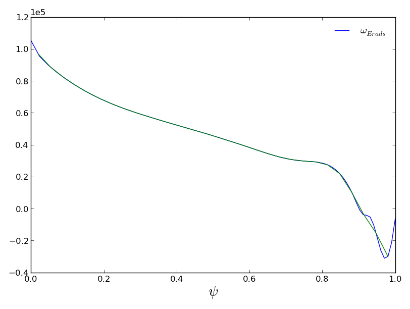
Note that the interpolator initialized the interpolation function on the first call, and saved it internally for the second.
Thats covers the basics. Test out the module yourself in ipython, getting familiar with things before moving on.
In this section, we will assume you have a pretty good hold on both python and the basic ploting functions of these modules.
Now that you use this module regularly, save yourself some time by placing the line:
from pypec import *
into your autoimport file located at ~/.ipython/profile_default/startup/autoimports.ipy
Right, now for the cool stuff:
One common need is to look at spectra. For this we want to utilize the full functionality of the data instances’ plot1d function.
>>> pspec, = read('examples/example_output_pmodb_n2.out')
Casting table 1 into Data object.
>>> f = pspec.plot1d('lagb','psi',x2rng=(0,8))
>>> f.axes[0].set_ylim(-0.005,0.005)
(-0.005, 0.005)
>>> f.savefig('examples/example_spectrum.png')
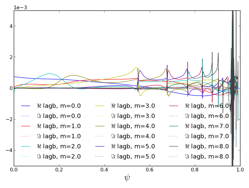
We knew it was one table, so we used the ”,” to automatically unpack returned list. We were then so familiar with the args and kwargs of the plotting function that we did not bother typing the names. If you do this, be sure you get the order consistent with the order given in the documentation “Definition” line (watch out for inconsistent “Docstring” listings).
Lets look through a huge file of first order perterbations we want to define some new data from the raw outputs, plot it, and save the results in a table
>>> pmodb, = read('examples/example_output_pmodb_fun_n2.out')
Casting table 1 into Data object.
WARNING: Reducing length of table from 2497639 to 1664452 by reducing x[0] by a factor of 3
>>> pmodb.y['cyltheta'] = np.arctan2(pmodb.y['z'],pmodb.y['r']-pmodb.params['R0'])
The data module automatically reduced the length of the data as it read it in order to spead up the reading and manipulation. If you need the full resolution, just set the rdim key word argument to infinity. Oh, and then we just added data!
>>> pmodb.y['kxprp'] = pmodb.y['Bkxprp']/pmodb.y['equilb']
>>> f1=pmodb.plot1d(['cyltheta','kxprp'],'theta',x2rng=0.16)
>>> f1.savefig('examples/example_pmodb.png')
>>> f1.printlines('examples/example_pmodb.dat',squeeze=True)
Wrote lines to examples/example_pmodb.dat
True
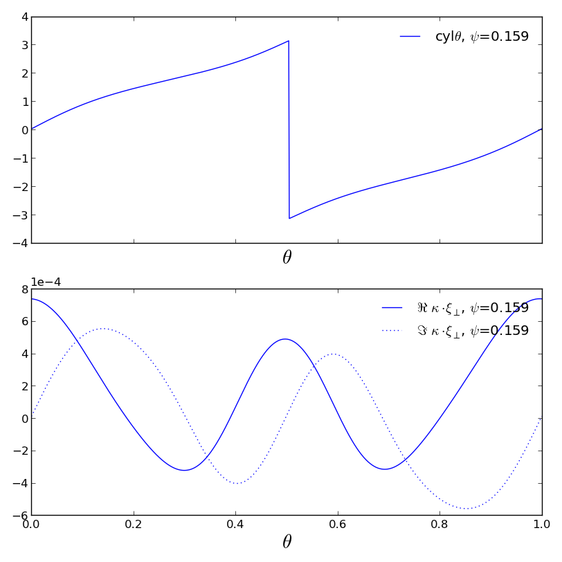
Thats it! Read the table with your favorit editor. It will probably need a little cleaning at the top since it tries to use the lengthy legend labels as column headers.
Lets look at some 2d data
>>> pb2, = read('examples/example_output_pbrzphi_n2.out')
Casting table 1 into Data object.
>>> f2 = pb2.plot2d('b_r')
Plotting real b_r.
Plotting imag b_r.
>>> f2.savefig('examples/example_pbrzphi.png')
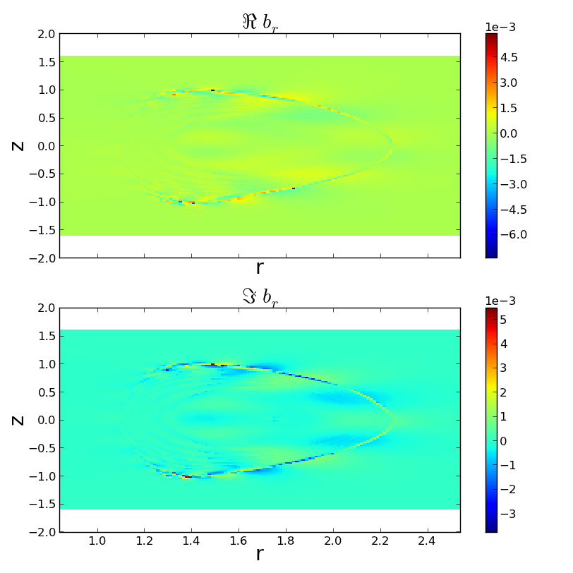
well that looks ugly! Lets stop the peak values from dominating dominating...
>>> f2 = pb2.plot2d('b_r',vmin=-1e-4,vmax=1e-4)
Plotting real b_r.
Plotting imag b_r.
If you are thinking “But those weren’t listed as keyword arguments!” then you have been glossing over the kwargs documentation. Most all pypec calls accept key word arguments for their root functions (in this case, pyplot.pcolormesh).
Finally, we want to make sure the aspect ratio is right
>>> f2 = pb2.plot2d('b_r',aspect='equal',vmin=-1e-4,vmax=1e-4)
Plotting real b_r.
Plotting imag b_r.
>>> f2.set_size_inches(6,13)
>>> f2.show()
>>> f2.savefig('examples/example_plot2d_pretty.png')
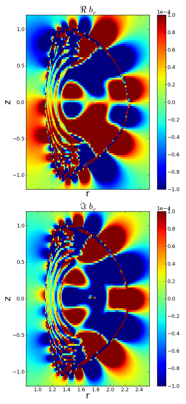
There. That looks better.
Note
These examples can be tested by developers using ipython in this directory as follows:
In [1]: import data,doctest
In [2]: doctest.testmod(data,verbose=True)
An emtpy class object with the following operations overloaded:
+,-,*,/,**
such that the operation is only performed on the attributes starting with .real_ and .imag_ and ending with r,z, or phi. If the two factors in the operation have different r or z attributes data is interpolated to the wider spaced axis.
Interpolate data to point(s).
Line plots of from 1D or 2D data.
Key Word Arguments:
- ynames : list
- Strings specifying dependent data displayed.
- xname : string
- The independent axis if 2D data.
- x1rng : optional
Valid formats are:
- x Plot single nearest point x-axis.
- (xmin,xmax) Plots all data in range (min,max).
- (xmin,xmax,n) Plots n evenly spaced points in range.
- x2rng : .
- Same as x1rng. Applicable to 2D or 3D data.
- x3rng : .
- Same as x2rng for 3D data only. Order of x is xnames with xname placed in front if given. kwargs : dict Valid matplotlib pyplot.plot keyword arguments.
Returns:
- f : figure
- poloidal cross sections of plasma response
Matplotlib pcolormesh or contour plots of 2D data.
Choose one of:
- “mesh” Use matplotlib pcolormesh to plot.
- “line” Use matplotlib contour to plot.
- “fill” Use matplotlib contourf to plot.
Three dimensional plots. Data with xnames r,z will be plotted with third dimension phi where Y = Re[y]cos(n*phi)+Im[y]sin(n*phi).
1D data > lines in a plane in 3-space. 2D data > z axis becomes y value 3D data > chosen display type
Must have mayavi.mlab module available in pythonpath.
Scatter plot display for non-regular data. Display mimics plot1d in t hat it displays a single independent axis. If is another independent axis exists, and is not sliced using one of the optional keyword arguments, it s represented as the color of the plotted symbols. If the data is 3D and unsliced, preference if given in order of xnames.
UNDER CONSTRUCTION
Return 1D data object from 2D. Method grids new data, so beware of loosing accuracy near rational surfaces.
Line plot of data gethered recursively from a dictionary containing multiple namelists or data objects.
Get the data from any ipec output as a list of python class-type objects using numpy.genfromtxt.
Recursively searches base directory for files with name filetype, reads them into python objects, and stores objects in a dictionary with directory names as keys.
Reads built-in geometric instances for the machine. These consist of surface objects, representing vessel walls, divertors, magnetic sensors, or any other 2D surface in the machine.
Write data object to file. The aim is to replicate the original file structure... the header text will have been lost in the read however, as will some column label symbols in the use of genfromtxt.
kwargs : dict. Passed to numpy.savetxt
This is a collection of wrapper functions for running DCON, IPEC, and PENT.
If run from the command line, this module will call an associated GUI.
This module is for more advanced operators who want to control/run the fortran package for DCON, IPEC, and PENT. To get started, lets explore the package
>>> gpec.
gpec.InputSet       gpec.join           gpec.optimize       gpec.run
gpec.bashjob        gpec.namelist       gpec.optntv         gpec.subprocess
gpec.data           gpec.np             gpec.os             gpec.sys
gpec.default        gpec.ntv_dominantm  gpec.packagedir     gpec.time
many of these are simply standard python modules imported by gpec lets submit a full run in just 4 lines: steal the settings from a previous run (leaving run director as deafult)
>>> new_inputs = gpec.InputSet(indir='/p/gpec/users/nlogan/data/d3d/ipecout/145117/ico3_n3/')
change what we want to
>>> new_inputs['dcon']['DCON_CONTROL']['nn']=2
>>> new_dir = new_inputs.indir[:-2]+'2'
DOUBLE CHECK THAT ALL IPUTS ARE WHAT YOU EXPECT (not shown here) and submit the job to the cluster.
>>> gpec.run(loc=new_dir,**new_inputs.infiles)
Running the package using this module will
You will not that there is significant oportunity for overwriting files, and the user must be responsible for double checking that all inputs are correct and will not result in life crushing disaster for themselves or a friend when that super special file gets over-written.
Class designed to hold the standard inputs for a run.
Run pent for series of scaled omega_phi/omega_E/omega_D values. User must specify full path to all files named in pent.in input file located in the base directory. Note that the rotation profile is scaled be manipulating omega_E on each surface to obtain the scaled roation.
Python wrapper for running ipec package multiple times in a search for the normalized spectrum that maximizes NTV.
- maxiter : int.
- Maximum number of iterations.
- loc : str.
- Directory location for run.
- rundir : str.
- IPEC package directory with executables and .dat files.
- kwargs : dict.
- namelist instance(s) written to <kwarg>.in file(s).
Note
Namelists taken from (in order of priority): 1) Key word arguments 2) .in files from loc 3) .in files from rundir
Python wrapper for running ipec package.
Note
Namelists taken from (in order of priority): 1) Key word arguments 2) .in files from loc 3) .in files from rundir
This module provides pythonic tools for reading and writing fortran namelists.
This module can be used to convert FORTRAN namelist files into python ordered dictionary type objects. The individual namelists are capitalized and their paramters are left as written. The actual parameter is thus stored two levels deep in the dictionary.
>>> nl=read('examples/example_namelist.in')
>>> nl.keys()
['IPEC_INPUT', 'IPEC_CONTROL', 'IPEC_OUTPUT', 'IPEC_DIAGNOSE']
>>> nl['IPEC_CONTROL'].keys()
['resp_index', 'sing_spot', 'reg_flag', 'reg_spot', 'chebyshev_flag', 'nche']
>>> nl['IPEC_CONTROL']['reg_spot']
0.05
The parameters can be changed, added, or deleted as in any python dictionary.
>>> nl['IPEC_CONTROL']['reg_spot'] = 0.01
>>> nl['IPEC_CONTROL']['reg_spot']
0.01
>>> del nl['IPEC_CONTROL']['nche']
>>> nl['IPEC_CONTROL'].keys()
['resp_index', 'sing_spot', 'reg_flag', 'reg_spot', 'chebyshev_flag']
>>> nl['IPEC_CONTROL']['nche'] = 30
The resulting namelists can then be re-written in ASCII format for use with the FORTAN codes.
>>> write(nl,'examples/example_namelist_edit.in')
True
Note
These examples can be tested by developers using ipython as follows:
In [1]: import pypec.namelist,doctest
In [2]: doctest.testmod(pypec.namelist,verbose=True)
Bases: object
Read in a file. Must have namelists in series, not embedded. Assumes name of list preceded by ‘&’ and list ends with ‘’.
Note
The returned dict is actually “OrderedDict” type from collections module. If returning an object, the object is un-ordered.
Write namelist object to file for fortran interface.
Collection of modified matplotlib functions and objects.
Plot complex arguments.
>>> f,ax = subplots()
>>> lines = ax.plot(np.arange(10)*(1+0.5j),label='test')
>>> pyplot.show()
Automatically resize plots to fit labels.
>>> xlbl = ax.set_xlabel('X AXIS')
Plot huge data sets quickly.
>>> x = np.linspace(0,9,1e5)
>>> data = np.arange(1e5)/1.5e4+(np.random.rand(1e5)-0.5)
>>> newline = ax.plot(x,data,label='large data set')
This plots a line capped at 1000-pts by default. The maximum number of points is maintained as you manipulate the axis, so zooming in will provide you with new points and increased detail until the window samples fewer than that many points in the orginal data. The first two lines, for instance, contain only their original 10 points (not 1000 interpolated points).
Modified pyplot colorbar for default use_gridspec=True.
ORIGINAL DOCUMENTATION
Add a colorbar to a plot.
Function signatures for the pyplot interface; all but the first are also method signatures for the colorbar() method:
colorbar(**kwargs)
colorbar(mappable, **kwargs)
colorbar(mappable, cax=cax, **kwargs)
colorbar(mappable, ax=ax, **kwargs)
arguments:
- mappable
- the Image, ContourSet, etc. to which the colorbar applies; this argument is mandatory for the colorbar() method but optional for the colorbar() function, which sets the default to the current image.
keyword arguments:
- cax
- None | axes object into which the colorbar will be drawn
- ax
- None | parent axes object from which space for a new colorbar axes will be stolen
- use_gridspec
- False | If cax is None, a new cax is created as an instance of Axes. If ax is an instance of Subplot and use_gridspec is True, cax is created as an instance of Subplot using the grid_spec module.
Additional keyword arguments are of two kinds:
axes properties:
Property Description orientation vertical or horizontal fraction 0.15; fraction of original axes to use for colorbar pad 0.05 if vertical, 0.15 if horizontal; fraction of original axes between colorbar and new image axes shrink 1.0; fraction by which to shrink the colorbar aspect 20; ratio of long to short dimensions anchor (0.0, 0.5) if vertical; (0.5, 1.0) if horizontal; the anchor point of the colorbar axes panchor (1.0, 0.5) if vertical; (0.5, 0.0) if horizontal; the anchor point of the colorbar parent axes colorbar properties:
Property Description extend [ ‘neither’ | ‘both’ | ‘min’ | ‘max’ ] If not ‘neither’, make pointed end(s) for out-of- range values. These are set for a given colormap using the colormap set_under and set_over methods. extendfrac [ None | ‘auto’ | length | lengths ] If set to None, both the minimum and maximum triangular colorbar extensions with have a length of 5% of the interior colorbar length (this is the default setting). If set to ‘auto’, makes the triangular colorbar extensions the same lengths as the interior boxes (when spacing is set to ‘uniform’) or the same lengths as the respective adjacent interior boxes (when spacing is set to ‘proportional’). If a scalar, indicates the length of both the minimum and maximum triangular colorbar extensions as a fraction of the interior colorbar length. A two-element sequence of fractions may also be given, indicating the lengths of the minimum and maximum colorbar extensions respectively as a fraction of the interior colorbar length. spacing [ ‘uniform’ | ‘proportional’ ] Uniform spacing gives each discrete color the same space; proportional makes the space proportional to the data interval. ticks [ None | list of ticks | Locator object ] If None, ticks are determined automatically from the input. format [ None | format string | Formatter object ] If None, the ScalarFormatter is used. If a format string is given, e.g. ‘%.3f’, that is used. An alternative Formatter object may be given instead. drawedges [ False | True ] If true, draw lines at color boundaries. The following will probably be useful only in the context of indexed colors (that is, when the mappable has norm=NoNorm()), or other unusual circumstances.
Property Description boundaries None or a sequence values None or a sequence which must be of length 1 less than the sequence of boundaries. For each region delimited by adjacent entries in boundaries, the color mapped to the corresponding value in values will be used.
If mappable is a ContourSet, its extend kwarg is included automatically.
Note that the shrink kwarg provides a simple way to keep a vertical colorbar, for example, from being taller than the axes of the mappable to which the colorbar is attached; but it is a manual method requiring some trial and error. If the colorbar is too tall (or a horizontal colorbar is too wide) use a smaller value of shrink.
For more precise control, you can manually specify the positions of the axes objects in which the mappable and the colorbar are drawn. In this case, do not use any of the axes properties kwargs.
It is known that some vector graphics viewer (svg and pdf) renders white gaps between segments of the colorbar. This is due to bugs in the viewers not matplotlib. As a workaround the colorbar can be rendered with overlapping segments:
cbar = colorbar()
cbar.solids.set_edgecolor("face")
draw()
However this has negative consequences in other circumstances. Particularly with semi transparent images (alpha < 1) and colorbar extensions and is not enabled by default see (issue #1188).
Downsample line data for increased plotting speed.
Function to connect key_press_event events from matplotlib to custom functions.
Matplotlib defaults (may be changed in matplotlibrc):
keymap.fullscreen : f # toggling keymap.home : h, r, home # home or reset mnemonic keymap.back : left, c, backspace # forward / backward keys to enable keymap.forward : right, v # left handed quick navigation keymap.pan : p # pan mnemonic keymap.zoom : o # zoom mnemonic keymap.save : s # saving current figure keymap.quit : ctrl+w # close the current figure keymap.grid : g # switching on/off a grid in current axes keymap.yscale : l # toggle scaling of y-axes (‘log’/’linear’) keymap.xscale : L, k # toggle scaling of x-axes (‘log’/’linear’) keymap.all_axes : a # enable all axes
My custom function mapping:
popaxes : n #Creates new figure with current axes tighten : t #Call tight_layout bound method for figure
Re-create a given axis in a new figure. This allows, for instance, a subplot to be moved to its own figure where it can be manipulated and/or saved independent of the original.
- Arguments:
- ax : obj.
- An initialized Axes object
- Key Word Arguments:
- fig: obj.
- A figure in which to re-create the axis
- geometry : tuple.
- Axes geometry of re-created axis
Print all data in line plot(s) to text file.The x values will be taken from the line with the greatest number of points in the (first) axis, and other lines are interpolated if their x values do not match. Column lables are the line labels and xlabel.
Matplotlib subplots with default sharex=True.
- Additional Key Word Arguments:
- powlim : tuple.
- Axis labels use scientific notion above 10^power.
- useOffset : bool.
- Axis labels use offset if range<<average.
Accepts standargs args and kwargs for pyplot.subplots.
ORIGINAL DOCUMENTATION
Create a figure with a set of subplots already made.
This utility wrapper makes it convenient to create common layouts of subplots, including the enclosing figure object, in a single call.
Keyword arguments:
- nrows : int
- Number of rows of the subplot grid. Defaults to 1.
- ncols : int
- Number of columns of the subplot grid. Defaults to 1.
- sharex : string or bool
- If True, the X axis will be shared amongst all subplots. If True and you have multiple rows, the x tick labels on all but the last row of plots will have visible set to False If a string must be one of “row”, “col”, “all”, or “none”. “all” has the same effect as True, “none” has the same effect as False. If “row”, each subplot row will share a X axis. If “col”, each subplot column will share a X axis and the x tick labels on all but the last row will have visible set to False.
- sharey : string or bool
- If True, the Y axis will be shared amongst all subplots. If True and you have multiple columns, the y tick labels on all but the first column of plots will have visible set to False If a string must be one of “row”, “col”, “all”, or “none”. “all” has the same effect as True, “none” has the same effect as False. If “row”, each subplot row will share a Y axis. If “col”, each subplot column will share a Y axis and the y tick labels on all but the last row will have visible set to False.
- squeeze : bool
If True, extra dimensions are squeezed out from the returned axis object:
- if only one subplot is constructed (nrows=ncols=1), the resulting single Axis object is returned as a scalar.
- for Nx1 or 1xN subplots, the returned object is a 1-d numpy object array of Axis objects are returned as numpy 1-d arrays.
- for NxM subplots with N>1 and M>1 are returned as a 2d array.
If False, no squeezing at all is done: the returned axis object is always a 2-d array contaning Axis instances, even if it ends up being 1x1.
- subplot_kw : dict
- Dict with keywords passed to the add_subplot() call used to create each subplots.
- fig_kw : dict
- Dict with keywords passed to the figure() call. Note that all keywords not recognized above will be automatically included here.
Returns:
fig, ax : tuple
- fig is the matplotlib.figure.Figure object
- ax can be either a single axis object or an array of axis objects if more than one subplot was created. The dimensions of the resulting array can be controlled with the squeeze keyword, see above.
Examples:
x = np.linspace(0, 2*np.pi, 400)
y = np.sin(x**2)

# Just a figure and one subplot
f, ax = plt.subplots()
ax.plot(x, y)
ax.set_title('Simple plot')

# Two subplots, unpack the output array immediately
f, (ax1, ax2) = plt.subplots(1, 2, sharey=True)
ax1.plot(x, y)
ax1.set_title('Sharing Y axis')
ax2.scatter(x, y)

# Four polar axes
plt.subplots(2, 2, subplot_kw=dict(polar=True))

# Share a X axis with each column of subplots
plt.subplots(2, 2, sharex='col')

# Share a Y axis with each row of subplots
plt.subplots(2, 2, sharey='row')

# Share a X and Y axis with all subplots
plt.subplots(2, 2, sharex='all', sharey='all')
# same as
plt.subplots(2, 2, sharex=True, sharey=True)