ElVis
1. Programming Interface
Application programs can send data and set the
appearance of the graph. Programming interfaces for different
languages are available:
1.1 Developing Applets with ElVis
Java applets can incorporate ElVis graphs.
The classes for creating graphs are in elvis.jar. The
applet and its classes can be stored in a separate .jar file.
The applet is launched from an HTML file such as:
<applet
code="EApplet.class"
codebase="classes/"
archive="eapplet.jar,
elvis.jar"
width="1024"
height="768">
<param name="type"
value="application/x-java-bean;version=1.3">
</applet>
A sample applet is in EApplet.java and archived in eapplet.jar.
2. Graph Components
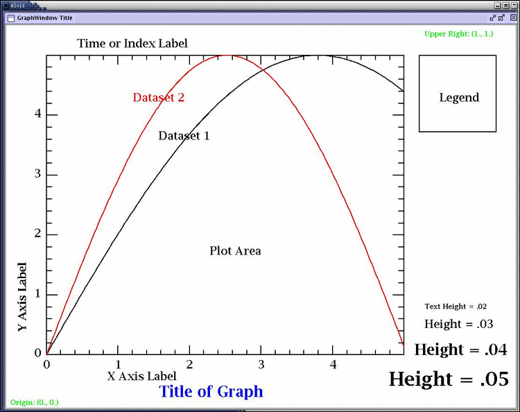
The elements of a graph are shown in the diagram
above. The graph contains:
- Plot Area
- X Axis with label
- Y Axis with label
- Title
- Index Label
- Text Labels
- Legend
The coordinate system of the graph has its origin
(0., 0.) at the lower left corner. The coordinates of the
upper right corner are (1., 1.). The location and size of
elements, including the height of text labels, is specified in this
coordinate system. All the elements scale continuously and
uniformly when the size of the graph is changed.
The default layout for a graph is shown in the
diagram above. The axes labels, title, and index label are
automatically drawn if the application program specifies a text
string. If no string is specified then no text is drawn.
Additional labels can be drawn anywhere within the graph.
Labels are clipped to the edges of the graph. Portions
of a label that extend beyond an edge of the graph are not seen.
Plot Area
The size and location of the plot area can be
controlled through the API. The default plot area shown in
the diagram is used if the application does not specify a plot
area.
The datasets are drawn within the plot area.
A dataset is equivalent to a "function" in a "multigraph"
drawn by the rplot program. A graph contains one or more
datasets. Each dataset is drawn in a different color.
Markers can be drawn at the location of data points.
When datasets are not indexed they are all drawn in the plot
area at the same time.
A dataset represents a function at a specific
index value. For time indexed data, the function at each time
step is added to the graph as a separate indexed dataset. If
the datasets are indexed in time or some other variable then only
the dataset for the current index value is drawn. Each indexed
dataset is drawn with the same color. The datasets are
displayed sequentially or animated continuously in index order.
The user interface has controls for incrementing or
decrementing the index value and animating the playback.
X Axis, Y Axis
The X axis is drawn along the bottom of the
graph. A label is automatically drawn below the numbers.
The Y axis is drawn along the left edge of the
graph. A label is automatically drawn to the left of the
numbers.
Major ticks and minor ticks are automatically drawn
along the axis based on the range of the data. The tick
locations are computed in ElVis so the tick numbers increment
equally. Tick numbers contain up to 3 digits, a decimal point,
and a negative sign when needed. If all the numbers for an
axis can be represented in 3 digits then algebraic numbering style
is used. If not, then the numbers are automatically shown in
scientific notation. The mantissa is drawn next to the major
tick and the exponent string is appended to the axis label.
There is an option to draw grid lines across the graph at
major tick locations.
The application program can set the spacing of
the ticks to be linear or logarithmic. The default is linear.
Title
A title label is automatically positioned below
the plot area.
Index Label
Datasets can be indexed by time or a user
specified quantity. Indexed datasets are displayed sequentially or
animated continuously. The index number is drawn along with
the specified text.
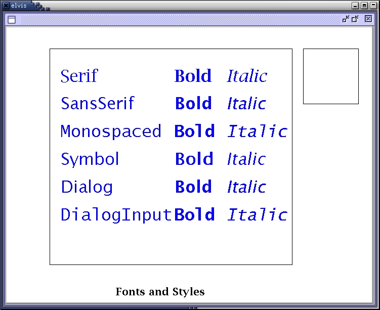
Text Labels
Additional labels can be drawn anywhere in the
graph. The application sets the location color, font, style,
and size of the label. The figure below shows fonts and styles
that are available.
Legend
A legend is drawn when 2 or more datasets are
plotted. Each entry in the legend contains the name of the
dataset and the style and color of its plot.
3. GraphWindow
Graphs are located within GraphWindows. A
GraphWindow contains a grid of graphs. Each grid cell contains
1 graph as shown in the figure below.
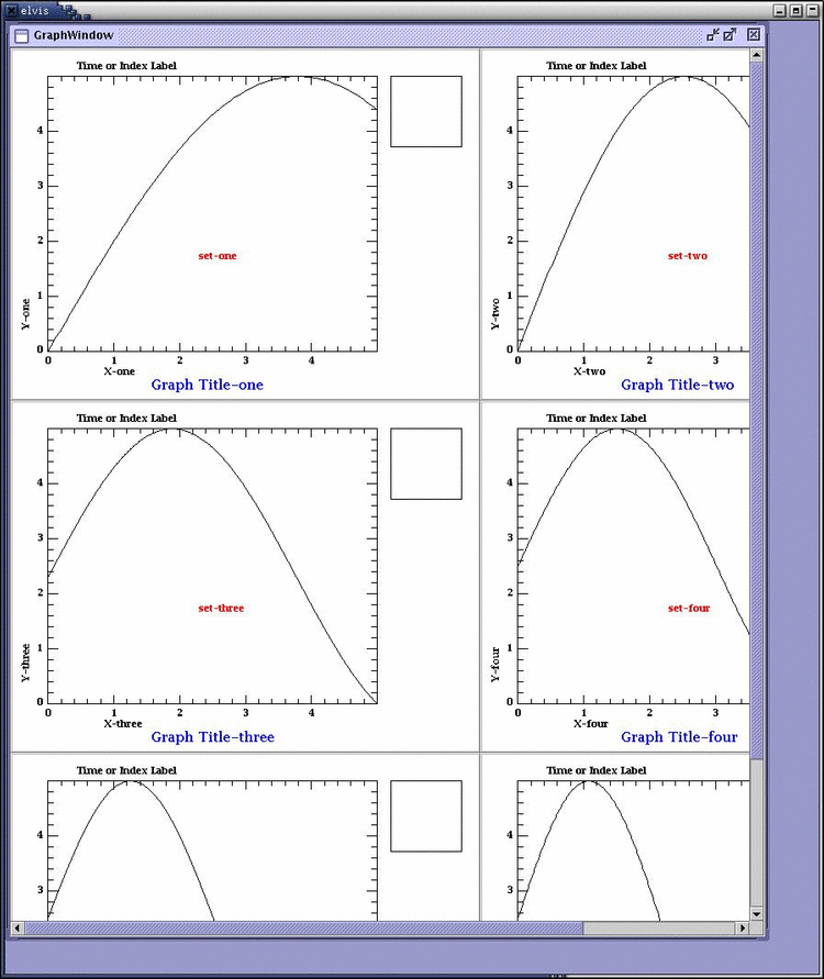
A GraphWindow has horizontal and vertical
scrollbars when the grid is bigger than the window. Dragging
the right edge of column changes the width of the column.
Dragging the bottom edge of a row changes the height of a row.
Dragging the lower right corner of a cell with mouse button 1
changes the column width and row height. Dragging the corner
with mouse button 3 maintains the aspect ratio of the graph in the
cell. The aspect ratio of other cells will change however.
The entire grid of graphs is shown when the
window is initially displayed. The menubar items for a
GraphWindow are:
Window-->Fit Scope Panel
- All of the graphs are shown, maintaining aspect ratio.
Window-->Fit Graph -
The graphs are resized so the upper left graph fills the
window.
Window-->Fill Graphs
- All of the graphs are shown and fill the window.
Window-->Print -
A PostScript file is created for each graph.
Window-->Close All -
All of the GraphWindows are removed.
The <----|----> button in the menubar
resizes all the graphs in a window. Clicking on the right half
of the button enlarges the graphs, while clicking on the left half
shrinks the graphs. The magnitude of the size change is
proportional to the horizontal distance from the center of the
button.
GraphWindows are automatically tiled as they are
added to the desktop window.
4. Interactive Features
4.1 Data Examination
4.1.1 Zoom and Translate the Data
The data drawn within the plot area can be
examined by zooming in. Drawing a zoom rectangle
with mouse button 1 (MB1) will set the zoom area. Press
MB1 within the plot area to set one corner of the rectangle and drag
the cursor to the opposite corner. The zoom rectangle is drawn
while maintaining the aspect ratio of the plot area. Releasing
MB1 applies the zoom.
Hold down the Ctrl key and press MB1 to start a
rectangle that will zoom out on the data.
Typing the = key zooms in. (The = key
increases the zoom and is a convenience for typing + to increase the
zoom.)
Typing the - key zooms out.
The 4 arrow keys translate the view of the data.
Move the cursor into the desired graph. Type the left,
right, up, or down arrow keys to translate the view of the data.
The view of the data can be reset from the
menubar: Graph-->Reset View.
The view of the selected graph can be applied to
all graphs in the GraphWindow from the menubar:
Graph-->Apply Scale All.
4.1.2 Display Data Values
To display data values, press MB1 above or below the plot area.
This will draw a vertical dashed line and display the X value
for that location in the data. A horizontal, color-coded
dashed line will be drawn for each intersecting dataset. The Y
value of the dataset will be displayed.
The data values will be displayed for each graph in the selected
GraphWindow. The graphs can be have different zoom and
translations.
The data values for indexed graphs can also be displayed while the
datasets are being animated.
4.2 Surface Plots
There are keyboard shortcuts for viewing options of surface plots:
Letter
Action
a
Draw lines, shaded polygons, and centroids.
f
Draw shaded polygons and the line segments
of each data set in the surface.
l
Draw polygon outlines and centroids.
p
Draw shaded polygons (default setting).
u
Toggles culling of back-facing polygons.
Turn off culling to see polygons from behind or below the surface.
w
Draw polygon outlines only.
/
Each / draws a polygon in depth
order. Type 0 to erase all; type 9 to display all.
5. Load gnuplot Files, Plots from Columns of
Data
ElVis can display a graph from a gnuplot command file containing
"plot" commands. The plot command references a text file
containing 2 or more columns of values. An example for the
plot command in a command file is:
plot "sim.dat" using
2:3 title "Simulation of Electron Density"
The filename is required and enclosed in quotation marks. The
filename is the first word after the plot command.
Each line in this text file contains 2 or more values, forming
columns of data. Any column can be used for either the X or
Y values. The column assignment is specified after the
keyword using. The example specifies column 2 as the
X values and column 3 as the Y values. If no column
assignment is made then column 1 is read as the X values and
column 2 is read as the Y values. The title of the graph is
(optionally) specified after the keyword title. The title
can be one or more words enclosed in quotation marks.
Multiple datasets can be plotted on one graph by having multiple
plot commands in the file. Each plot command should be on a
separate line in the command file. Alternatively, a plot
command can have more than one file by using a comma as a
separator:
plot "sim.dat" using 2:3,
"exp.dat" title "Comparison"
The command can continue on more than one line by ending each
line with \ as shown:
plot "sim.dat" using 2:3, \
"exp.dat" title "Comparison"
The commands for setting the X and Y axis labels are:
set xlabel "Your X Label"
set ylabel "Your Y Label"
Blank lines and comment lines starting with # are ignored.
For compatibility with the gnuplot parser, a style can be included
after the keyword using, such as: using 1:4 with lines, but it is
ignored when read into ElVis. The GraphEditor can be used to
display lines or points in a graph.
The command file is accessed from the menubar:
File-->Load File. This brings up a file selection
box. Set the Files of Type to gnuplot files. All files
except *.gw, *.nc, and *.cdf will be listed.