The data for this example are points in the continental U.S. with pressure readings - these data were supplied by Professor Alan Cline at the University of Texas.
The first plot was produced using the modified output file. Several modifications were made to the original file example9.dat produced by running the Fortran source. For example, mods were made to suppress drawing the Voronoi polygons and the natural neighbor circumcircles and centers.
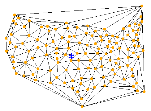
Of particular interest is the final section of the algorithmic data file where it has been indicated that we want to look at the natural neighbors of the coordinate (0.47, 0.31), but we only want to mark that point with an asterisk. Using the modified output file with nnalg produces the plot:

The blue asterisk marks the point at which we want to know the natural neighbors.
If we now want to see the natural neighbors of the point marked in the above plot, we change the appropriate flag, as described in the comments in the output data file, and get the plot:

The five blue dots surrounding the asterisk indicate the natural neighbors.
If displaying the second order natural neighbors is desired, changing the flag in the data file for that gives:

The blue dots now indicate all second order natural neighbors.
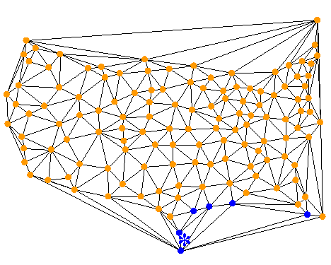
Changing the interpolated point of interest to (0.540E-00, 0.050E-00) [in the southern part of Texas] and plotting the first order neighbors produces the plot:

This illustrates that for interpolated values near the convex hull of a dataset where the convex hull differs significantly from the bounding polygon, the neighbor selection may be somewhat unsatisfactory. From the above plot we see that function values in Florida can contribute to an interpolated value in Texas. However, the effect is attenuated by the fact that the weights given to distant points are small, and this greatly reduces the influence of distant points.