GPU Programming at PPPL
Written by Eliot Feibush & Michael Knyszek
Introduction
Programming on Graphical Processing Units (GPUs) is incredibly
powerful in that it takes advantage of parallelism on a scale much
larger than most of today's supercomputers. Rather than relying on
massive amounts of machines which communicate with high-latency
connections, GPUs have a massive amount of tightly-knit, incredibly
lean cores that are heavily optimized for floating point operations.
What this means is that you can have millions of points on a grid
processed potentially hundreds of times faster than if you processed
them serially. A fuller, broader introduction to the power of GPUs
can be found in the following NVIDIA presentation for their new
Tesla GPUs:
Tesla GPU
Computing: Accelerating High Performance Computing
Although GPUs are fairly specialized in their computation, NVIDIA
has conveniently provided a list of just some of the many
applications of hardware accelerated computing ranging from finance
to science and research:
Popular GPU
Accelerated Applications
Table of Contents
GPU Devices at PPPL
cppg-6 Linux computer
An NVIDIA Tesla K20c GPU accelerator is installed in cppg-6.
The computer's original 525 watt power supply was replaced with a
1000 watt power supply to power the 233 watt board. The K20c
receives 80 watts from the PCI bus and 2 six pin power cables
deliver the rest of the power. There are 2496 CUDA cores in
this GPU. It contains 5 GB of on-board memory.
The computer is a Dell Precision T3500n with a 64-bit Intel Quad
Core Xeon processor. It contains 4 GB of host memory.
The graphics board is an NVIDIA Quadro FX 580 that drives 2 monitors
at 1600 x 1200 resolution each. The graphics board is also a
CUDA device with 32 cores. This computer mounts the PPPL file system
when you log in.
Note: it is currently running 64-bit Red Hat 5 kernel. This
computer mounts the PPL cluster file system so you can load PPL
modules as on portal.
ssh into cppg-6 to run the GPU software.
gpusrv GPU Cluster
gpusrv01
Two NVIDIA M2070 GPU accelerators are installed on gpusrv01.
These GPUs have 443 CUDA cores each and 5 GB of on-board memory.
gpusrv02
Two NVIDIA Tesla K20m GPU accelerators are installed in
gpusrv02. There are 2496 CUDA cores in each GPU and each GPU
contains 4.8 GB of on-board memory.
Run the "useg" or "use" command to be queued for access onto gpusrv.
Back to Top ➚
NVIDIA software
The NVIDIA SDK CUDA 5.0.35 (64-bit) software is installed in
/usr/pppl/cuda/cudatoolkit/5.0.35. The package includes nvcc
for cross compiling cuda programs to run on the K20.
At the Linux command line: module load cuda/5.0.35
/usr/bin/nvidia-smi -q
This program prints information about the NVIDIA
devices installed in the computer. There is a man page for
nvidia-smi or you can run nvidia-smi -h to see a list of
command line options.
Another sample program is in
/p/vis/cuda/samples/devicequerydrv. The deviceQueryDrv program there
prints information about the installed NVIDIA devices. The following
output is an example of running deviceQueryDrv
on cppg-6:
CUDA Device Query (Driver
API) statically linked version
Detected 2 CUDA Capable
device(s)
Device 0: "Tesla K20c"
CUDA Driver
Version:
5.0
CUDA Capability
Major/Minor version number: 3.5
Total amount of
global
memory:
4096 MBytes (4294967295 bytes)
(13) Multiprocessors
x (192) CUDA Cores/MP: 2496 CUDA Cores
GPU Clock
rate:
706 MHz (0.71 GHz)
Memory Clock
rate:
2600 Mhz
Memory Bus
Width:
320-bit
L2 Cache
Size:
1310720 bytes
Max Texture Dimension
Sizes
1D=(65536) 2D=(65536,65536) 3D=(4096,4096,4096)
Max Layered Texture
Size (dim) x layers
1D=(16384) x 2048, 2D=(16384,16384) x 2048
Total amount of
constant
memory:
65536 bytes
Total amount of
shared memory per block:
49152 bytes
Total number of
registers available per block: 65536
Warp
size:
32
Maximum number of
threads per multiprocessor: 2048
Maximum number of
threads per
block:
1024
Maximum sizes of each
dimension of a block: 1024 x 1024 x 64
Maximum sizes of each
dimension of a grid: 2147483647 x 65535
x 65535
Texture
alignment:
512 bytes
Maximum memory
pitch:
2147483647 bytes
Concurrent copy and
kernel
execution:
Yes with 2 copy engine(s)
Run time limit on
kernels:
No
Integrated GPU
sharing Host
Memory:
No
Support host
page-locked memory mapping:
Yes
Concurrent kernel
execution:
Yes
Alignment requirement
for
Surfaces:
Yes
Device has ECC
support:
Enabled
Device supports
Unified Addressing (UVA): No
Device PCI Bus ID /
PCI location
ID:
3 / 0
Compute Mode:
< Default (multiple host threads can use ::cudaSetDevice()
with device simultaneously) >
Device 1: "Quadro FX 580"
CUDA Driver
Version:
5.0
CUDA Capability
Major/Minor version number: 1.1
Total amount of
global
memory:
511 MBytes (536150016 bytes)
( 4) Multiprocessors
x ( 8) CUDA Cores/MP: 32 CUDA Cores
GPU Clock
rate:
1125 MHz (1.12 GHz)
Memory Clock
rate:
800 Mhz
Memory Bus
Width:
128-bit
Max Texture Dimension
Sizes
1D=(8192) 2D=(65536,32768) 3D=(2048,2048,2048)
Max Layered Texture
Size (dim) x layers
1D=(8192) x 512, 2D=(8192,8192) x 512
Total amount of
constant
memory:
65536 bytes
Total amount of
shared memory per block:
16384 bytes
Total number of
registers available per block: 8192
Warp
size:
32
Maximum number of
threads per multiprocessor: 768
Maximum number of
threads per
block:
512
Maximum sizes of each
dimension of a block: 512 x 512 x 64
Maximum sizes of each
dimension of a grid: 65535 x 65535 x 1
Texture
alignment:
256 bytes
Maximum memory
pitch:
2147483647 bytes
Concurrent copy and
kernel
execution:
Yes with 1 copy engine(s)
Run time limit on
kernels:
Yes
Integrated GPU
sharing Host
Memory:
No
Support host
page-locked memory mapping:
Yes
Concurrent kernel
execution:
No
Alignment requirement
for
Surfaces:
Yes
Device has ECC
support:
Disabled
Device supports
Unified Addressing (UVA): No
Device PCI Bus ID /
PCI location
ID:
2 / 0
Compute Mode:
< Default (multiple host threads can use ::cudaSetDevice()
with device simultaneously) >
It identifies the K20 as the first device. This is convenient
for the CUDA examples that appear later on in this document.
For more information about the GPU driver and NVIDIA software
included with the CUDA Toolkit, click on the course link below:
GPU
driver/CUDA
Back to Top ➚
Basic GPU Programming
Programming Course
More information on all three sections below can be found in a
larger course presentation which is very long, but contains
information on all 3 types of CUDA programming.
Click the link below to look at the full 107 slide course:
Full
3-part Introduction
Introduction to CUDA Libraries
In most cases, utilizing libraries built for performing various
mathematical operations and transformations may just be the easiest
way to take advantage of GPU parallelism.
CUDA Libraries such as:
- cuFFT - Fast Fourier Transforms Library
- cuBLAS - Complete BLAS Library
- cuSPARSE - Sparse Matrix Library
- cuRAND - Random Number Generation (RNG) Library
- NPP - Performance Primitives for Image & Video Processing
- Thrust - Templated C++ Parallel Algorithms & Data
Structures
- math.h - C99 floating-point Library (on the GPU)
can make paralleling codes for the GPU trivial by simply "dropping
in" library calls where you would otherwise perform certain
mathematical operations.
For a more detailed overview and some tips on how to get started
with the CUDA libraries, click on the course link below:
NVIDIA
CUDA Library Approach (First ~30 Pages of the Large Course Above)
For more information about the Thrust library specifically, check
out:
An Introduction to
the Thrust Parallel Algorithms Library
Introduction to OpenACC
For anyone familiar with OpenMP, working with OpenACC should be very
easy.
OpenACC is built on similar principles to OpenMP in that parallelism
is as simple as adding directives to your C/Fortran codes.
For a more detailed overview and some tips on how to get started
with OpenACC, click on the course link below:
GPU
Computing with OpenACC Directives
Introduction to CUDA C/C++
CUDA C/C++ is the most involved and most powerful form of GPU
programming of the above methods.
Built as an extension to C/C++, the language is easy to get started
with but the runtime can be tricky to master. However, it is
extremely powerful and offers the greatest degree of customization
and is the biggest opportunity for a speed boost in your code.
For a more detailed overview and some tips on how to get started
with CUDA C/C++, click on the course link below:
CUDA C/C++
Basics
Below is also a cheatsheet with some of the basic functions, syntax,
and ideas of CUDA C/C++:
CUDA C/C++ Cheatsheet
Back to Top ➚
Simple CUDA Examples
The NVIDIA training course provided several programming
examples.
Loading the cuda module should set up your include path and library
path for compiling and linking the example programs.
There are some sample CUDA programs in
/p/vis/cuda/samples/test.
The source code is in these files:
- addcuda.cu
- first.cu
- kernel.cu
- simple_gpu.cu
The Makefile will compile and link the codes so you can run the
examples:
- addcuda.out
- x.first
- x.hello_world
- x.simple_gpu
Back to Top ➚
More Sophisticated CUDA Examples
Generating Fractals
GPUs excel at performing many simultaneous computations that are mutually
independent. Perhaps one of the best examples of this is in
generating images of fractals since each point is calculated
independently, sharing only the same base equation. Two particularly
interesting fractals are those in the Mandelbrot set and the Julia
set, which are defined by the equation
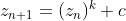
where z and c are complex numbers. Here is an example of what the
code below should produce:

(The short tutorial below does not run through coloring methods,
but to achieve the same coloring effect, take a rainbow palette
and use the output of the program to interpolate between colors on
a log2 scaling.)
To generate images of these fractals, we iteratively compute the
equation at discrete points and count the iterations it takes for
the absolute value of z to exceed a certain threshold. This is a
measure of how quickly the equation diverges and is interesting
because it produces fractal patterns. From this measure, we can then
color and draw the fractal. This is the simplest way to generate
fractals and is known as the Escape Time Algorithm, since it measure
how quickly the recursive equation "escapes" a certain bailout
radius (the threshold). If you are more interested in learning about
the math behind it, Wikipedia
actually has an excellent amount of information on the subject. This
example will instead focus on the GPU implementation aspect.
In this particular example, we need to define a few things. First of
all, we represent our image as simple an array of floating point
numbers in memory. Next, we need a way to pass the dimensions of the
image and what our "viewing window" is (the maximum and minimum
coordinates in the Argand plane to view). The solution to passing
all these arguments will be to use a special part of the GPU called
constant memory. It consists of a small amount of read-only
memory set aside for constants which are going to be accessed
frequently over all threads running in a kernel. We do this by first
defining a C struct with all our information, like so:
typedef struct {
    int width;
    int height;
    float x_max;
    float x_min;
    float y_max;
    float y_min;
    float c_re;
    float c_im;
} Dimensions;
Now we want to place an instance of our struct onto the GPU for
access. First, we need to declare some space in constant memory:
__constant__ Dimensions dev_d;
Second, we have to create our own instance, and then simply copy it
over! Supposing the variable "d" is a pointer to our host-side
Dimensions instance, we simply run the following code:
cudaMemcpyToSymbol(dev_d, d, sizeof(Dimensions), 0, cudaMemcpyHostToDevice);
One thing to keep in mind about constant memory is that for a warp
of threads (all the threads sharing a block) there is a 32-bit cache
for constant memory which can make reads of constant memory
extremely fast. The limitation here is that the cache size is
absolutely tiny. For a few constants, however, this can really
improve performance over reading the constant from global memory.
One should use constant memory with extreme care since, if used
improperly, could lead to a serious bottleneck in computation. A few
constants is okay, but having an array of hundreds of values would
destroy the purpose of constant memory.
An example of device code for a GPU implementation of a Mandelbrot
set fractal generator would look something like the following. Note:
we assume our equation here has k=2 which makes exponentiating the
complex number simple with just floats.
__global__ void mandelbrot(float *img) {

    // Get the current index based on thread and block number
    int index = threadIdx.x + blockIdx.x * blockDim.x;

    // Derive x and y points
    int Px = index % dev_d.width;
    int Py = index / dev_d.width;

    // Scale x-y coordinates into predefined scaling options
    // x0 and y0 are part of our constant c, in the mandelbrot case
    float x0 = (float)Px*(dev_d.x_max - dev_d.x_min)/((float)dev_d.width) + (float)dev_d.x_min;
    float y0 = (float)Py*(dev_d.y_max - dev_d.y_min)/((float)dev_d.height) + (float)dev_d.y_min;

    // Set some other variables, x and y are parts of a complex number, z0 = x + yi
    float x = 0;
    float y = 0;
    float tmp;
    int i = 0;

    // Perform the escape-time iteration scheme
    // BAILOUT_RADIUS is our threshold, MAX_ITER is how many iterations to
    // perform before giving up and assuming the equation converges.
    while(x*x + y*y < BAILOUT_RADIUS && i < MAX_ITER) {
        // Square z (x + iy) and add c (x0 + iy0)
        tmp = x*x - y*y + x0;
        y = 2*x*y + y0;
        x = tmp;
        ++i;
    }

    // Part of the "Normalized Iteration Count Algorithm", converts an integer iteration count into
    // a real number. Not particularly important, but useful for making coloring smoother.
    if(i == MAX_ITER) img[index] = (float) i;
    else img[index] = (float) i + 1.5 - log2(log2(x*x+y*y)/2);
}
All that is left to do is to follow the steps of setting up our
environment and running the kernel. If you have gone through the
course above, the following methods for setting up our image on the
GPU and copying it back should seem very familiar.
float *d_pixels; // pointer to image on device
float *h_pixels; // pointer to image on host

// size is the number of pixels in the image
h_pixels = (float*) malloc(size * sizeof(float)); // Allocate memory on host
cudaMalloc((void **) &d_pixels, size * sizeof(float)); // Allocate memory on device

// Start kernel, size is assumed divisible by THREADS_PER_BLOCK
mandelbrot <<< size/THREADS_PER_BLOCK, THREADS_PER_BLOCK >>> (d_pixels);

// Copy our processed image onto the host
cudaMemcpy(h_pixels, d_pixels, size * sizeof(float), cudaMemcpyDeviceToHost);

// Force the host to wait for the device to finish so we do not write garbage data into the image
cudaDeviceSynchronize();

// ... Insert Image Writing Code Here ...
With this simple setup, you can implement a whole host of
variations. For example, you could generate Julia set fractals, make
fractal movies by altering parameters slightly, such as the constant
for the Julia set or the exponent "k" which the equation uses.
All these features and more are implemented and can be examined by
simply going into /u/mknyszek/cuda/fractals and having a
look at the files.
Here are some videos of these features in action:
Back to Top ➚
2D Fluid Simulation
Another useful application of GPU programming is fluid simulations.
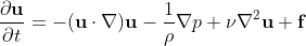
In this particular example, we will be working with the
Navier-Stokes Equations for incompressible, constant density fluids:

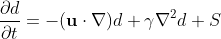
And this tutorial will introduce an "ink" whose density will not be
constant and will be moved about by the fluid. The density of the
"ink" can be described by the following equation:

Like the previous fractals example, this tutorial will not dive too
deeply into the mathematics. However, it is important to understand
what numerical methods we are using here. The methods described here
will be based upon the paper Stable Fluids
(Stam, 1999) (ACM Entry) for
some calculations, and we will simply take advantage of finite
difference forms for other calculations. To summarize, the idea here
is that we perform advection, diffusion, and the addition of body
forces to a velocity with non-zero divergence. Afterwards, we
calculate the pressure (which can be represented as a Poisson
equation) at each point on the grid using a Jacobi solver, and
subtract the gradient at each point from the our velocity to project
it onto a space where it has a divergence of zero, satisfying the
second equation above. We will also use the stable method for
calculating advection as described in Stable Fluids,
Stam, 1999, which involves moving backwards in time rather
than forwards, which will be explained further down.
Some more important details about this implementation are:
- Numerical Details
- We will use a grid size that is one-to-one with pixels.
- Pixel edges are considered boundaries, whereas data
(velocity, substance) will be at the center of each pixel.
- For simplicity's sake, we will assume a non-viscous fluid
(so, no diffusion of velocity) and we will not allow the
"ink" to diffuse either.
- Treatment of Boundary Conditions
- We will solve the Navier-Stokes equations enforcing solid
wall or "no-slip" boundary conditions for velocity, and pure
Neumann boundary conditions for pressure.
- Because boundary values are largely separate from the
primary operations, we will only perform operations on
values inside the boundary cells, which are the cells on the
outside (indices 0, width-1, and 0, height-1 on the x and y
axes respectively.)
- Technical Details
- Similarly to the fractals example, we will be using a
Dimensions structure loaded into constant memory (see
above), but with slightly different parameters.
- We shall split the components of velocity, u and v, into
separate arrays.
- As with the fractals example, we will "flatten" our image
into a 1D array and use 1D arrays for all quantities.
- Due to the nature of some of the operations performed, we
will have to keep a buffer array of previous values for most
quantities. These previous array values will be stored in
arrays with the suffix "old".
- As is common with most CG applications, we work assuming
that 0,0 is the top-left corner, and moving downwards and
right is a positive x,y increase.
Our overall approach will look something like this:
- Add Body Forces to Velocity and Add "ink" from Sources
- Advect Velocity and Density ("ink")
- Calculate Divergence of Velocity
- Solve Pressure Poisson Equation using the Jacobi Method: Ax=b
where x is pressure and b is velocity divergence.
- Use Pressure to Correct/Project Velocity to be Divergence-Free
- Write Density ("ink") Values to Image
First, we define our Dimensions struct and constant memory
allocation:
typedef struct {
    int width;
    int height;
    int steps;
    float timestep;    // Timestep in Seconds
    float dissipation; // Mass Dissipation Constant (how our "ink" dissipates over time). Set to 1 for no dissipation, 0.995 tends to look nice though.
} Dimensions;

...

__constant__ Dimensions ddim;
Next, we will define all our kernels and methods. By design, and
unlike the fractals example, we will have many kernels that will be
performing operations over a large number of points in parallel.
Think of these operations as "slab" operations, performing
calculations on large areas of memory simultaneously.
Organizing the code this way with many kernels keeps things
organized with only minor overhead. Potentially, you could gain a
speed boost by performing many of these operations in a single
kernel, but you have to be careful to make sure you call __syncthreads()
the proper amount of times. We use this multiple kernel technique
for simplicity and clarity.
Add Forces/Sources
This is a very simple procedure. We simply add whatever our force or
source amount is multiplied by the size of our timestep to each
point in our grid.
__global__ void add_source(float *d, float *s) {
    int i = threadIdx.x + blockIdx.x * blockDim.x;
    int width = ddim.width;
    int height = ddim.height;
    int px = i % width;
    int py = i / width;

    // Skip Boundary values
    if(px > 0 && py > 0 && px < width-1 && py < height-1)
    {
        // Add source each timestep
        d[i] += ddim.timestep * s[i];
    }
}
The first argument is left as just "d" because we will use this same
kernel to add our body forces to the horizontal and vertical
components of velocity, in addition to "ink" density.
Advection
The advection kernel is significantly more complicated. As described
in Stable
Fluids (Stam 1999), trying to advect density or velocity
forward in time (by taking the previous velocity at each point and
following it to a new point and putting that velocity there) is
unstable and leads to oscillations in the calculation over time.
Instead, here we take the velocity at each point, follow it in its
opposite direction, and find the velocity at that point using
bilinear interpolation. We then update the velocity at our current
point with that interpolated velocity.
Conveniently, it turns out that the unstable method is also
unsuitable for GPU programming because we can end up with multiple
threads trying to write to the same memory location, which can cause
serious problems! With this method, each thread safely updates only
its own dedicated grid point while only reading other, old grid
points.
__global__ void advect(float *dold, float *d, float *u, float *v, float md) {
    int i = threadIdx.x + blockIdx.x * blockDim.x;
    int width = ddim.width;
    int height = ddim.height;
    int px = i % width;
    int py = i / width;

    int px0, py0, px1, py1;
    float x, y, dx0, dx1, dy0, dy1;

    // Skip Boundary values
    if(px != 0 && py != 0 && px != width-1 && py != height-1)
    {
        // Move "backwards" in time
        x = px - ddim.timestep * (width-2)  * u[i]; // Multiply by the width of the grid not including the boundary
        y = py - ddim.timestep * (height-2) * v[i]; // Multiply by the height of the grid not including the boundary

        // Clamp to Edges, that is, if the velocity goes over the edge, clamp it to the boundary value
        if (x < 0.5) x = 0.5; if (x > width - 1.5)  x = width - 1.5;
        if (y < 0.5) y = 0.5; if (y > height - 1.5) y = height - 1.5;

        // Setup bilinear interpolation "corner points"
        px0 = (int) x; px1 = px0 + 1; dx1 = x - px0; dx0 = 1 - dx1;
        py0 = (int) y; py1 = py0 + 1; dy1 = y - py0; dy0 = 1 - dy1;

        // Perform a bilinear interpolation
        d[i] = dx0 * (dy0 * dold[px0 + width*py0] + dy1 * dold[px0 + width*py1]) +
               dx1 * (dy0 * dold[px1 + width*py0] + dy1 * dold[px1 + width*py1]);

        // Multiply by the mass dissipation constant
        d[i] *= md;
    }

    return;
}
Here again, "d" is a placeholder variable since we will use both
velocities and density in its place. "dold" refers to the array of
previous values and "d" refers to the array storing new values.
Divergence
For calculating the divergence, we use the finite difference method
for the divergence of a vector field. In our case, delta x and delta
y are both 1 (since we define the grid size to be one-to-one with
pixels). Thus, our kernel is simply:
__global__ void divergence(float *u, float *v, float *div) {
    int i = threadIdx.x + blockIdx.x * blockDim.x;
    int width = ddim.width;
    int height = ddim.height;
    int px = i % width;
    int py = i / width;

    // Skip Boundary values
    if(px > 0 && py > 0 && px < width-1 && py < height-1)
    {
        float u_l = u[i-1];
        float u_r = u[i+1];
        float v_t = v[px + (py-1)*width];
        float v_b = v[px + (py+1)*width];

        // Calculate divergence using finite difference method
        // We multiply by -1 here to reduce the number of negative multiplications in the pressure calculation
        div[i] = -0.5 * ((u_r - u_l)/(width-2) + (v_b - v_t)/(height-2));
    }
}
Pressure
We implement here a kernel for one iteration of the Jacobi solver
for pressure, which can be represented a Poisson equation. Since the
step of each solver depends on the last, we have to perform some
pointer manipulations and boundary updates in between iterations,
which is why we implement it this way.
__global__ void pressure(float *u, float *v, float *p, float *pold, float *div) {
    int i = threadIdx.x + blockIdx.x * blockDim.x;
    int width = ddim.width;
    int height = ddim.height;
    int px = i % width;
    int py = i / width;

    // Skip Boundary values
    if(px > 0 && py > 0 && px < width-1 && py < height-1)
    {
        // left, right, top, bottom neighbors
        float x_l = p[i-1];
        float x_r = p[i+1];
        float x_t = p[px + (py-1)*width];
        float x_b = p[px + (py+1)*width];
        float b = div[i];

        // Jacobi method for solving the pressure Poisson equation
        pold[i] = (x_l + x_r + x_t + x_b + b) * 0.25; // Here b is positive because of the extra negative sign in the divergence calculation
    }
}
Normally the Jacobi method is one of the methods that converges the
most slowly. However, on the GPU each Jacobi iteration is incredibly
cheap since the entire pressure array is updated nearly
simultaneously. It is possible to implement the red-black
Gauss-Siedel relaxation algorithm to solve for pressure, however
this is more unnecessarily complex for the sake of this tutorial.
From a GPU programming perspective, each step is very similar and no
real benefit is gained from that implementation. Regardless, for an
interesting look into the method, see this publication
from the Universidade da Beira Interior.
Projection/Correction
Nothing very interesting occurs in this kernel. Essentially, the
finite difference method for taking the gradient of a scalar field
is used (with dx and dy being 1) to get the gradient of pressure.
Each component of the gradient is then subtracted from the
respective velocity component.
__global__ void correction(float *u, float *v, float *p) {
    int i = threadIdx.x + blockIdx.x * blockDim.x;
    int width = ddim.width;
    int height = ddim.height;
    int px = i % width;
    int py = i / width;

    // Skip Boundary values
    if(px > 0 && py > 0 && px < width-1 && py < height-1) {

        // left, right, top, bottom neighbors
        float p_l = p[i-1];
        float p_r = p[i+1];
        float p_t = p[px + (py-1)*width];
        float p_b = p[px + (py+1)*width];

        // Find the gradient and perform the correction/projection
        u[i] -= 0.5*(p_r - p_l)*(width-2);
        v[i] -= 0.5*(p_b - p_t)*(height-2);
    }
}
Boundary Conditions
In order to enforce our defined boundary conditions (no-slip and
pure Neumann), we have to have kernels to occasionally update the
boundary conditions of both velocity components and pressure.
For velocity, we want the edge between the boundary grid points and
the closest inner grid point to have a horizontal velocity of zero
for vertical edges, and a vertical velocity of zero for horizontal
edges. Simply by looking at the finite difference method, we see we
can do this by setting the boundary grid point velocities to be
negative that of the velocity directly inside.
__global__ void velocity_bc(float *u, float *v) {
    int i = threadIdx.x + blockIdx.x * blockDim.x;
    int width = ddim.width;
    int height = ddim.height;
    int px = i % width;
    int py = i / width;

    // Skip Inner Values
    if(px == 0)
    {
        u[i] = -u[i+1];
        v[i] =  v[i+1];
    }
    else if(py == 0)
    {
        u[i] =  u[px + (py+1)*width];
        v[i] = -v[px + (py+1)*width];
    }
    else if(px == width-1)
    {
        u[i] = -u[i-1];
        v[i] =  v[i-1];
    }
    else if(py == height-1)
    {
        u[i] =  u[px + (py-1)*width];
        v[i] = -v[px + (py-1)*width];
    }
}
For pressure, we want the edge between the boundary grid points and
the closest inner grid point to have a derivative of zero with
respect to the normal. By using the finite difference method for the
derivative of pressure in the direction of the normal, we see that
our pressure on the boundary grid point needs to be set equal to the
pressure value of the closest inner grid point.
__global__ void pressure_bc(float *p) {
    int i = threadIdx.x + blockIdx.x * blockDim.x;
    int width = ddim.width;
    int height = ddim.height;
    int px = i % width;
    int py = i / width;

    // Skip Inner Values
    if(px == 0)
    {
        p[i] = p[i+1];
    }
    else if(py == 0)
    {
        p[i] = p[px + (py+1)*width];
    }
    else if(px == width-1)
    {
        p[i] = p[i-1];
    }
    else if(py == height-1)
    {
        p[i] = p[px + (py-1)*width];
    }
}
Putting It All Together
Finally, we just have to put this all together in the step order we
described above (with a few extra pointer swaps, boundary value
updates, and memory updates in between).
For reference, we set up all our variables first, like we did for
the fractals example:
// Full size of arrays, including boundaries
int size = dim->width * dim->height;

// size is necessarily divisible by a constant THREADS_PER_BLOCK defined elsewhere
int blocks = size/THREADS_PER_BLOCK;

//
// All Device Pointers
//

//velocity and pressure
float *u, *v, *p;
float *uold, *vold, *pold;
float *utemp, *vtemp, *ptemp; // temp pointers, DO NOT INITIALIZE

//divergence of velocity
float *div;

//density
float *d, *dold, *dtemp;
float *map;

//sources
float *sd, *su, *sv;

...

//
// Allocate memory for most arrays
//

...

// Initialize our "previous" values of density and velocity to be all zero
cudaMemset(uold, 0, size * sizeof(float));
cudaMemset(vold, 0, size * sizeof(float));
cudaMemset(dold, 0, size * sizeof(float));

// Host density copy, you can initialize this if you'd like, then copy it to dold
map = (float *) malloc(size * sizeof(float));

// Create the sources using some arbitrary source creation function
// that you wish to use
sd = create_source();
su = create_source();
sv = create_source();
Now, we can begin our main loop, putting all our kernels to good
use:
for(t = 0; t < steps; ++t) {

    //add sources to velocity (body force)
    add_source <<< blocks, THREADS_PER_BLOCK >>> (uold, su);
    add_source <<< blocks, THREADS_PER_BLOCK >>> (vold, sv);

    //add sources to density
    add_source <<< blocks, THREADS_PER_BLOCK >>> (dold, sd);

    //advect horizontal and vertical velocity components
    advect <<< blocks, THREADS_PER_BLOCK >>> (uold, u, uold, vold, 1);
    advect <<< blocks, THREADS_PER_BLOCK >>> (vold, v, uold, vold, 1);

    //advect density
    advect <<< blocks, THREADS_PER_BLOCK >>> (dold, d, u, v, 0.995);

    //call kernel to compute boundary values and enforce boundary conditions
    velocity_bc <<< blocks, THREADS_PER_BLOCK >>> (u, v);

    //call kernel to compute the divergence (div)
    divergence <<< blocks, THREADS_PER_BLOCK >>> (u, v, div);

    //reset pressure to 0 <- This is our initial guess to the Jacobi solver
    cudaMemset(p, 0, size * sizeof(float));

    //for each Jacobi solver iteration, 80 tends to be enough iterations to get convergence or close enough
    for (i = 0; i < 80; ++i)
    {
        //call kernel to compute pressure
        pressure <<< blocks, THREADS_PER_BLOCK >>> (u, v, p, pold, div);

        //swap old and new arrays for next iteration
        ptemp = pold; pold = p; p = ptemp;

        //call kernel to compute boundary values and enforce boundary conditions
        pressure_bc <<< blocks, THREADS_PER_BLOCK >>> (p);
    }

    //call kernel to correct velocity
    correction <<< blocks, THREADS_PER_BLOCK >>> (u, v, p);

    //call kernel to compute boundary values and enforce boundary conditions
    velocity_bc <<< blocks, THREADS_PER_BLOCK >>> (u, v);

	//copy density image back to host and synchronize
    cudaMemcpy(map, d, size * sizeof(float), cudaMemcpyDeviceToHost);
    cudaDeviceSynchronize();
    /*************************************************
     *                                               *
     *    Write to Image Here, Or Anywhere Really    *
     *                                               *
     ************************************************/

    //swap old and new arrays for next iteration
    utemp = uold; uold = u; u = utemp;
    vtemp = vold; vold = v; v = vtemp;
    dtemp = dold; dold = d; d = dtemp;
}
And that's a 2D fluid simulation based on the Navier-Stokes equation
on the GPU! Like it was mentioned above, you can add diffusive
effects to both the density and velocity giving the fluid some sense
of viscosity and allowing the "ink" to disperse more realistically.
One downfall of this method is that due to numerical error, you tend
to lose the extra vorticity in the movement of the fluid, but you
can restore this using vorticity confinement methods.
Overall, compared to traditional serial methods, this tends to run
much faster, and the bottleneck still tends to be the writing of
images as opposed to the actual calculations. If you would like to
view the full source code, go to /u/mknyszek/cuda/nsflow and
all the files should be there.
For some examples of what this simulation code has produced, take a
look at these videos:
Back to Top ➚
Debugging CUDA Code
Debugging CUDA code can seem daunting at first because at first it
may seem almost impossible to look at values on GPU memory without
first copying the values back to the CPU. Luckily, NVIDIA provides
several methods for debugging CUDA code and handling errors.
Before you get started, for the most detailed results with NVIDIA
CUDA debugging tools, make sure to compile your code with the -G
flag in addition to the -g flag (which is the standard gcc flag for
compiling with debugging information).
printf Usage
On newer GPUs (such as the ones we have at the lab) you can actually
use printf statements in device code to find out values at a certain
time. The only issue is that when a kernel runs, it cannot print out
values in real-time. When using printf, be wary of the fact that
anything printing will only appear after the kernel terminates.
During kernel execution the string is shoved into a buffer which is
then flushed at kernel termination. This can sometimes make
debugging very tedious as you get inundated with statements printed
to the command line simultaneously.
Of course, you can always isolate a certain thread and only print
values from that thread, but in the end that can be a lot of wasted
effort because the range of values you can see is now very narrow
and it won't bring you to the root of the problem.
cuda-gdb
NVIDIA has developed an extension to gdb to help diagnose and
eliminate bugs in CUDA programs. Simply run cuda-gdb in the same way
you would run gdb, and cuda-gdb will give you a plethora of
information about your program as its running, including kernel
launches and any errors or warnings related to CUDA runtime
functions.
cuda-gdb works identically to gdb and lets you view values in global
memory as well as set breakpoints in your device code just as you
would with any other C/C++ program.
While cuda-gdb can really save you a few hours of debugging your
device code, it can sometimes act strangely with host code. It is
recommended that when you have problems with your host code, stick
to using only gdb as it is much more reliable.
cuda-memcheck
If you fear that your program is starting to do strange things with
GPU memory and other memory errors are occurring that are not made
obvious using cuda-gdb, NVIDIA has also provided another program
called cuda-memcheck. Run it on your program by specifying your
program as an argument to cuda-memcheck and it will generate a nice
report if it finds any fatal memory errors.
HANDLE_ERROR Macro
Although NVIDIA includes a hefty error handling system for CUDA
runtime subroutines, it can get very tedious to use for every single
instance of a CUDA runtime function you wish to check.
This tool in particular is not a tool created by NVIDIA but rather
by developers who use it to handle errors easily for the purposes of
debugging. Simply define the following function and macro at the top
of your file:
static void HandleError(
cudaError_t err, const char *file, int line ) {
if (err != cudaSuccess) {
printf( "%s in %s at line %d\n",
cudaGetErrorString( err ), file, line );
exit( EXIT_FAILURE );
}
}
#define HANDLE_ERROR( err ) (HandleError( err, __FILE__, __LINE__
))
This macro now makes handling CUDA runtime errors very easy. Simply
wrap your CUDA runtime functions with the macro like so:
HANDLE_ERROR( cudaMalloc((void
**) &d, size * sizeof(float)) );
Back to Top ➚
Profiling CUDA Code
When your code is complete and working well, you may wish to
identify bottlenecks in running time and optimize the code to
squeeze out as much GPU performance as possible.
NVIDIA also has a pair of tools for profiling: one for the command
line and one with an Eclipse-based GUI. Before using either of these
tools, make sure you first compile your code with the -pg flag.
nvprof
This is NVIDIA's counterpart to the well-known C program profiler
gprof. nvprof is excellent for performing quick profiling checks on
your code to ensure that time is being expended where you expect it
to. Its very lightweight and handy, and in addition can be run on any
program that creates CUDA kernels. This even includes programs which
use OpenACC or CUDA Python and it can be extremely helpful for
determining where exactly a CUDA kernel is being launched and for
what.
One particularly helpful flag for nvprof is --print-gpu-trace which
prints a detailed GPU stack trace with all function calls, what GPU
they are running on, and their dimensions.
Another helpful flag is --output-profile which generates a file
detailing the profile, which can be later imported back into nvprof,
or perhaps nvvp.
If you find that your program uses significant CPU time as well,
using a combination of nvprof and gprof can give you a nice look
into where the most time is being spent.
nvvp
nvvp is the NVIDIA Visual Profiler. Simply create a new session,
specify the command line arguments and working directory of your
properly compiled program, and it will generate very detailed
reports regarding the performance of your program. There exist
additional options to only profile certain portions of your program
too, among other things. Those accustomed to Eclipse should find
that this tool is very easy to use and incredibly useful.
Back to Top ➚
Tips & Tricks
Below is a collection of tips & tricks that have been mostly
found through experience and can come in handy if/when CUDA C/C++
does not behave as expected.
- Pay special care to not read from uninitialized device
memory. While this is good practice for any memory read, this is
especially important when it comes to the GPU because it can
lead to values accidentally persisting and data becoming
corrupt.
- When attempting to port code over to the GPU, try first to
have it parallelized and working using some other method such as
OpenMP or MPI. When the operations are already paralellized, it
is much easier to make the port because the code is better
structured for it.
- The saying "premature optimization is the root of all evil"
also applies to GPU programming. It is better to have something
working than to try to over-optimize it the first time around.
Even unoptimized GPU code tends to be significantly faster than
serial code.
- Do not forget that CUDA C/C++ comes with its own math
library, including things such as hypot() (which will compute
the sqrt(x^2 + y^2)). Built-in functions tend to be much faster
and hypot(), for example, is guaranteed to only overflow if the
result would overflow, meaning that the built-in library tends
to be much safer.
- Too many math operations slowing you down? Try compiling with
--fast-math. Your program will lose numerical accuracy, but will
get a significant performance boost.
- CUDA C/C++ comes with vector types (float2, float3, int4,
double3, etc.) with their own constructors (make_())
that guarantee memory alignment. Use them, but use them with
caution. Not much documentation exists so you may find
yourself wondering if an array or matrix of these vector types
is worth the headache.
Back to Top ➚