3.3 QuadMesh Objects

Currently only PyGist supports QuadMeshes.

Instantiation

from quadmesh import *

qm = QuadMesh ( <keylist>)

Description

The QuadMesh class provides a means of encapsulating information about two-dimensional, quadrilateral meshes and plotting the information connected with these meshes in various ways. Information can be plotted as contour lines, filled contours, or filled cells; different regions of the mesh can be plotted with different characteristics; and vector fields can be plotted on all or part of the mesh. The keyword arguments for QuadMesh objects are:

x, y, ireg, boundary, boundary_type, boundary_color, regions, region, inhibit, tri, z, levels, filled, contours, edges, ecolor, ewidth, vx, vy, type, color, hide, width, marks, marker

QuadMesh, like all other 2d classes, also has methods set and new.

Keyword Arguments

x and y, matching two-dimensional sequences of floating point values. These arguments are required and give the coordinates of the nodes of the mesh.

ireg, the region map: optional two-dimensional sequence of integer values with the same dimensions as x and y, giving positive region numbers for the cells of the mesh, zero where the mesh does not exist. The first row and column of ireg should be zero (although these values will be ignored), since there are one fewer cells in each direction than there are nodes.

boundary = 0/1; 0: plot entire mesh; 1: plot only the boundary of the selected region(s).

boundary_type, boundary_color: these matter only if boundary = 1, and tell how the boundary will be plotted ("solid", "dash", "dot", "dashdot", "dashdotdot", or "none") and what its color will be.

region = n: if n = 0, plot entire mesh; if any other number, plot the region specified (according to the settings in ireg).

regions = [r₁, r₂,...]: this option allows the user to specify to a QuadMesh a list of Region objects (see Section 3.4 "Region Objects" on page 33) to plot. Each object may have different plotting characteristics (see Section "Examples" on page 34). Only regions r₁, r₂, ... will be plotted.

regions = "all" (the default): plot all regions of the mesh.

inhibit = 0/1/2; 0: Plot all mesh lines. 1: Do not plot the (x [:, j], y [:, j]) lines; 2: Do not plot the (x [i,:], y[i,:]) lines; 3: If boundary = 1, do not plot boundaries. (Default: 0.) 0, 1, and 2 only apply if edges = 1.

tri, optional two-dimensional sequence of values with the same dimensions as ireg, triangulation array used for contour plotting.

z = optional two-dimensional sequence of floating point values. Has the same shape as x and y. If present, the contours of z will be plotted (default: 8 contours unless levels (see below) specifies otherwise), or a filled mesh will be plotted if filled = 1. In the latter case, z may be one smaller than x and y in each direction, and represents a zone-centered quantity.

levels = either:

(1) optional one-dimensional sequence of floating point values. If present, a list of the values of z at which you want contours; or

(2) if a single integer, represents the number of contours desired. They will be computed (at equal levels) by the graphics.

filled = 0/1: If 1, plot a filled mesh using the values of z if contours = 0, or plot filled contours if contours = 1 (this option is not available at the time of writing of this manual, but will be added soon). If z is not present, the mesh zones will be filled with the background color, which allows plotting of a wire frame. (default value: 0.)

contours = 0/1: if 1, contours will be plotted if filled = 0, and filled contours will be plotted if filled = 1 (this option is not available at the time of writing of this manual, but will be added soon). contours normally defaults to 0, but will default to 1 if edges = 0 and filled = 0.

The table below summarizes the effects of these two keywords (assuming z is present):

TABLE 3. filled and contours

	contours = 0	contours = 1
filled = 0	k and/or l lines if edges = 1	contour lines
filled = 1	filled mesh ("bg" fill if z = None)	filled contours

edges, if nonzero, draw a solid edge around each zone. If edges = 0 and filled = 0, draw contour lines. (Default value: 0.)

ecolor, ewidth--the color and width of the mesh lines when filled = 1 and edges is nonzero.

vx, vy--optional two-dimensional sequences of floating point values. Has the same shape as x and y. If present, represents a vector field to be plotted on the mesh.

scale = floating point value. When plotting a vector field, a conversion factor from the units of (vx, vy) to the units of (x, y). If omitted, scale is chosen so that the longest vectors have a length comparable to a ``typical'' zone size.

z_scale = specifies "log", "lin", or "normal" for how z is to be plotted.

type, color, width, label, hide, and marks are as for curves.

marker is different, since you would not want to specify the same marker for all contours in a contour plot. Instead, you can use marker to designate the letter (or number) which you want to mark the lowest contour curve; then the remaining contours will be lettered or numbered consecutively from that point on.

Methods new and set are as in the Curve class. Remember the warning about set: very little error checking is done, so if you are not careful, you could assign conflicting values to keywords.

Examples

The following Python code computes a mesh and some data on the mesh to be used in the QuadMesh examples which follow. This same code will be assumed in the examples given in the next section on Regions. Note the import statements, which bring in the necessary name spaces to do the computations.

from quadmesh import *

from graph2d import *

from Ranf import *

from Numeric import *

from shapetest import *

s = 1000.

kmax = 25 # The mesh is going to be 25 by 35

lmax = 35 # (24 cells by 34)

xr = multiply.outer ( arange (1, kmax + 1, typecode = Float),

ones (lmax))

yr = multiply.outer ( ones (kmax), arange (1, lmax + 1,

typecode = Float))

zt = 5. + xr + .2 * random_sample (kmax, lmax)

rt = 100. + yr + .2 * random_sample (kmax, lmax)

z = s * (rt + zt)

z = z + .02 * z * random_sample (kmax, lmax)

z [3:10, 3:12] = z [3:10, 3:12] * .9

z [5, 5] = z [5, 5] * .9

z [17:22, 15:18] = z [17:22, 15:18] * 1.2

z [16, 16] = z [16, 16] * 1.1

# Define a vector field on the mesh:

ut = rt/sqrt (rt ** 2 + zt ** 2)

vt = zt/sqrt (rt ** 2 + zt ** 2)

# Define the region map:

ireg = multiply.outer ( ones (kmax), ones (lmax))

# The first row and column should be 0:

ireg [0:1, 0:lmax]=0

ireg [0:kmax, 0:1]=0

ireg [1:15, 7:12]=2

ireg [1:15, 12:lmax]=3

# Create a void in the mesh:

ireg [3:7, 3:7]=0

3.3.1 Plots of Mesh Lines

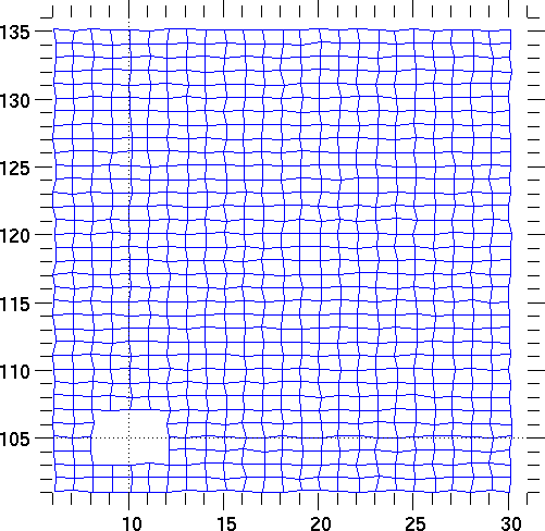
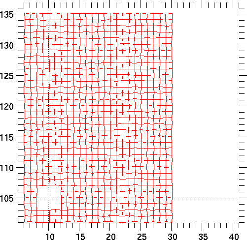
The following code plots the mesh lines in three different ways, as described in the comments:

# Instantiate a QuadMesh object qm with the mesh defined

# by zt, rt, and ireg; its lines to be of width 1,

# and blue in color:

qm = QuadMesh (x = zt, y = rt, ireg = ireg, width = 1.,

color = "blue")

# Create a Graph2d object gr with a reference to qm:

gr = Graph2d (qm)

# Plot the graph. Note the void area in the graph.

gr.plot ()

# Change to a red-colored mesh:

qm.set (color = "red", width = 1.)

# Change the plot so that the x and y axes have the same

# scale (the mesh will appear narrower)¹:

gr.change_plot(xyequal = 1)

# Change the color of the mesh to yellow:

qm.set (color = "yellow")

# Let Gist calculate the x and y scales depending

# on the data:

gr.change_plot(xyequal = 0)

3.3.2 Contour Plots

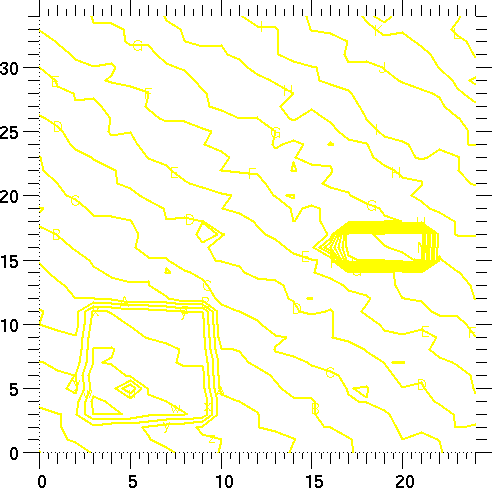
In this example, we create a uniform 25 by 35 mesh, and do a contour plot of the values of z computed above. Then we go back to the (xr, yr) mesh used above. We use the same Graph2d object as the preceding example, deleting object 1 and then adding the new QuadMesh object each time.

sh = shape (z)

sh1 = sh[0]

sh2 = sh[1]

x = multiply.outer (arange (sh1, typecode = Float),

ones (sh2, Float))

y = multiply.outer (ones (sh1, Float),

arange (sh2, typecode = Float))

# qm2 will have twenty yellow contour levels

# with default labels (capital letters):

qm2 = QuadMesh (z = z, y = y, x = x, color = "yellow",

width = 3., levels = 20, marks = 1)

# Delete object 1 (the only one) from gr:

gr.delete (1)

# Add the new object to gr, and plot it:

gr.add (qm2)

gr.plot ()

# Now change back to (xr, yr), mesh plotted with dashes

# in the foreground color:

qm2 = QuadMesh (z = z - z[kmax / 2, lmax / 2] ,

y = yr, x = xr, type = "dash",

color = "fg", levels = 20, width = 2., marks = 1)

gr.delete (1)

gr.add (qm2)

gr.plot ()

# Now plot the same thing as a filled contour plot:

qm2.set(filled=1)

gr.plot ()

# Next, plot the default number of contours (8) in

# purple with width 3; start marking with letter "O":

qm2 = QuadMesh (z = z, y = yr, x = xr , color = "purple" ,

marks = 1, marker = "O", width = 3.)

gr.delete (1)

gr.add (qm2)

gr.plot ()

# Finally, plot four specified contour levels (three

# contours) in cyan, width 3:

qm2 = QuadMesh (z = z, y = yr, x = xr , color = "cyan" ,

marks = 1, width = 3., levels = [0., max (ravel (z)) / 4.,

3. * max (ravel (z)) / 4., 7. * max (ravel (z)) / 8.])

gr.delete (1)

gr.add (qm2)

gr.plot ()

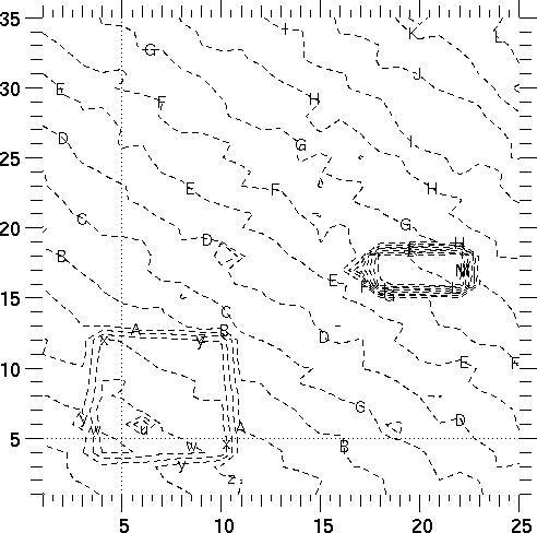
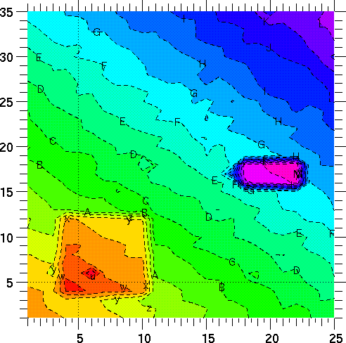
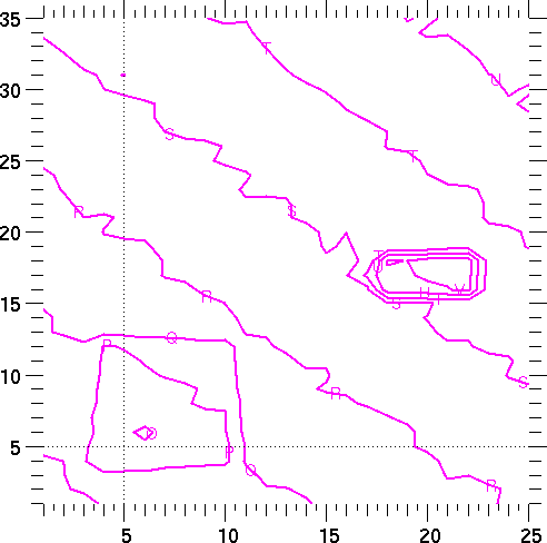
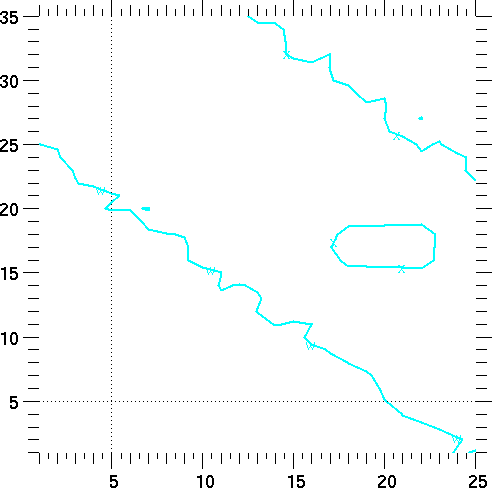
Note: the Graph method change_plot changes the appearance of the existing plot; there is no need to issue another plot call. See "Description" on page 75