[Top] [Prev] [Next] [Bottom]
7.5 At Last - the 3-D Plotting Functions
7.5.1 plwf: plot a wire frame
Calling Sequence
plwf (z [, y, x] [, <keylist>] )
Description
plwf plots a 3-D wire frame of the given 2-D array z. If x and y are given, then they must be the same shape as z or else len (x) should be the first dimension of z and len (y) the second. If x and y are not given, they default to the first and second indices of z, respectively. plwf calls clear3 before putting the plot command on the display list, which means that PyGist can only show one wire frame at a time using this function. (See pl3tree for graphs with multiple components).
plwf accepts the following keyword arguments:
fill, shade, edges, ecolor, ewidth, cull, scale, cmax
A description of the keywords follows:
fill: optional colors to use (default is to make zones have background color), same dimension options as for z argument to plf function, i. e., it should be the same dimension as the mesh (vertex-centered values) or one smaller in each dimension (cell-centered values).
shade: set non-zero to compute shading from the current 3-D lighting sources.
edges: default is 1 (draw edges), but if you provide fill colors, you may set to 0 to supress the edges.
ecolor, ewidth: color and width of edges.
cull: default is 1 (cull back surfaces), but if you want to see the ``underside'' of the model, set to 0.
scale: by default, z is scaled to ``reasonable'' maximum and minimum values related to the scale of (x, y). This keyword alters the default scaling factor, in the sense that scale = 2.0 will produce twice the z-relief of the default scale = 1.0.
cmax: the ambient keyword in light3 can be used to control how dark the darkest surface is; use this to control how light the lightest surface is. The lightwf routine can change this parameter interactively.
Examples
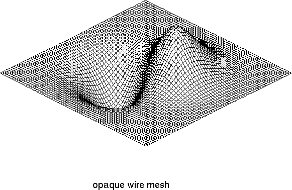
The following example computes the information for a surface with a peak and a valley, and then plots the resulting wire frame with various options. In the first case, we see simply an opaque wire frame.
- set_draw3_ (0)
- x = span (-1, 1, 64, 64)
- y = transpose (x)
- z = (x + y) * exp (-6.*(x*x+y*y))
- orient3 ( )
- light3 ( )
- plwf (z, y, x)
- [xmin, xmax, ymin, ymax] = draw3(1)
- limits (xmin, xmax, ymin, ymax)
- plt("opaque wire mesh", .30, .42)
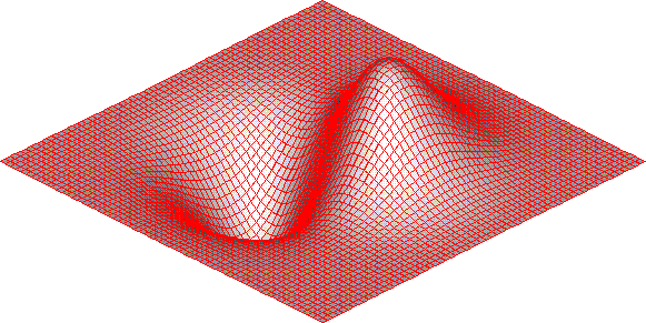
Next, we see the same surface shaded from a default light source (roughly over the viewer's right shoulder) and with the mesh lined in red.
- plwf(z,y,x,shade=1,ecolor="red")
- [xmin, xmax, ymin, ymax] = draw3(1)
- limits (xmin, xmax, ymin, ymax)
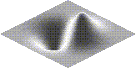
Finally, the following sequence plots the same surface with no edges, and with lighting coming from the back.
- plwf(z,y,x,shade=1,edges=0)
- light3 ( diffuse=.1, specular=1., sdir=array([0,0,-1]))
- [xmin, xmax, ymin, ymax] = draw3(1)
- limits (xmin, xmax, ymin, ymax)
7.5.2 pl3surf: plot a 3-D surface
Calling Sequence
pl3surf (nverts, xyzverts [, values] [, <keylist>])
Description
Perform simple 3-D rendering of an object created by slice3 (possibly followed by slice2). nverts and xyzverts are polygon lists as returned by slice3, so xyzverts is sum (nverts)-by-3, where nverts is a list of the number of vertices in each polygon. If present, the values should have the same length as nverts; they are used to color the polygon. If values is not specified, the 3-D lighting calculation set up using the light3 function will be carried out. Keywords cmin and cmax as for plf, pli, or plfp are also accepted. (If you do not supply values, you probably want to use the ambient keyword to light3 instead of cmin here, but cmax may still be useful.)
pl3surf calls clear3 before putting the plot command on the display list, which means that PyGist can only show one surface at a time using this function. (See pl3tree below for graphs with multiple components).
Example
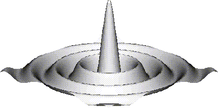
The following example is the familiar sombrero function. The first few lines of code compute its value.
- nc1 = 100
- nv1 = nc1 + 1
- br = - (nc1 / 2)
- tr = nc1 / 2 + 1
- x = arange (br, tr, typecode = Float) * 40. / nc1
- y = arange (br, tr, typecode = Float) * 40. / nc1
- z = zeros ( (nv1, nv1), Float)
- r = sqrt (add.outer ( x ** 2, y **2)) + 1e-6
- z = sin (r) / r
In order to use pl3surf, we need to construct a mesh using mesh3. The way we shall do that is to define a function on the 3d mesh so that the sombrero function is its 0-isosurface.
- z0 = min (ravel (z))
- z0 = z0 - .05 * abs (z0)
- maxz = max (ravel (z))
- maxz = maxz + .05 * abs (maxz)
- zmult = max (max (abs (x)), max (abs (y)))
- dz = (maxz - z0)
- nxnynz = array ( [nc1, nc1, 1], Int)
- dxdydz = array ( [1.0, 1.0, zmult*dz], Float )
- x0y0z0 = array ( [float (br), float (br), z0*zmult], Float )
- meshf = zeros ( (nv1, nv1, 2), Float )
- meshf [:, :, 0] = zmult*z - (x0y0z0 [2])
- meshf [:, :, 1] = zmult*z - (x0y0z0 [2] + dxdydz [2])
Finally, we create the mesh and call the plotting functions.
- m3 = mesh3 (nxnynz, dxdydz, x0y0z0, funcs = [meshf])
- fma ()
- # Make sure we don't draw till ready
- set_draw3_ (0)
- pldefault(edges=0)
- [nv, xyzv, col] = slice3 (m3, 1, None, None, value = 0.)
- orient3 () # (default orientation)
- pl3surf (nv, xyzv)
- lim = draw3 (1)
- dif = 0.5 * (lim [3] - lim [2])
- # dif is used to compress the y scale a bit.
- limits (lim [0], lim [1], lim [2] - dif, lim [3] + dif)
- palette ("gray.gp")
The graph that results from this sequence of code is on the next page.
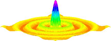
This next sequence of functions uses slice3mesh to draw the same surface; this time the polygons that make up the surface are colored according to height (using the rainbow palette).
- # Try new slicing function to get color graph
- [nv, xyzv, col] = slice3mesh (nxnynz [0:2], dxdydz [0:2],
- x0y0z0 [0:2], zmult * z, color = zmult * z)
- pl3surf (nv, xyzv, values = col)
- lim = draw3 (1)
- dif = 0.5 * (lim [3] - lim [2])
- limits (lim [0], lim [1], lim [2] - dif, lim [3] + dif)
- palette ("rainbow.gp")
7.5.3 pl3tree: add a surface to a plotting tree
pl3tree accepts surfaces and slices of surfaces in the slice2/slice3 format, and, as its name suggests, builds a b-tree. Its purpose is to attempt to analyze multiple surface plots in such a way as to determine the order of plotting, so that hidden portions of the surfaces will be graphed first, and this covered by later portions. pl3tree may be called multiple times to build plots of arbitrary complexity.
Calling Sequence
- pl3tree (nverts, xyzverts [, values] [, <keylist>])
Description
pl3tree accepts the following keywords:
- plane, cmin, cmax, split
pl3tree adds the polygon list specified by nverts (number of vertices in each polygon) and xyzverts (3-by-sum (nverts) vertex coordinates) to the currently displayed b-tree. If values is specified, it must have the same dimension as nverts, and represents the color of each polygon. If values is not specified, then the polygons are assumed to form an isosurface which will be shaded by the current 3-D lighting model; the isosurfaces are at the leaves of he b-tree, sliced by all of the planes. If plane (in the format returned by a call to plane3) is specified, then the xyzverts must all lie in that plane, and that plane becomes a new slicing plane in the b-tree.
Each leaf of the b-tree consists of a set of sliced isosurfaces. A node of the b-tree consists of some polygons in one of the planes, a b-tree or leaf entirely on one side of that plane, and a b-tree or leaf on the other side. The first plane you add becomes the root node, slicing any existing leaf in half. When you add an isosurface, it propagates down the tree, getting sliced at each node, until its pieces reach the existing leaves, to which they are added. When you add a plane, it also propagates down the tree, getting sliced at each node, until its pieces reach the leaves, which it slices, becoming the nodes closest to the leaves.
This structure is relatively easy to plot, since from any viewpoint, a node can always be plotted in the order from one side, then the plane, then the other side.
If keyword split is set nonzero (the default), then this routine assumes a ``split palette''; the current palette will be ``split'' or truncated so that its colors are numbered 0 to 99, while colors 100 to 199 will be greyscale. Colors for the values will be scaled to fit from color 0 to color 99, while the colors from the shading calculation will be scaled to fit from color 100 to color 199. (If values is specified as an unsigned char array (Python typecode "b"), however, it will be used without scaling.) You may specifiy a cmin or cmax keyword to affect the scaling; cmin is ignored if values is not specified (use the ambient keyword from light3 for that case).
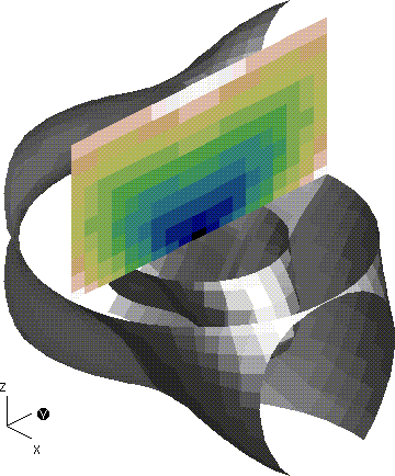
Example
In the following example, nx, ny, and nz are each 20. First we compute the mesh and some data on the mesh.
- xyz = zeros ( (3, nx, ny, nz), Float)
- xyz [0] = multiply.outer ( span (-1, 1, nx),
- ones ( (ny, nz), Float))
- xyz [1] = multiply.outer ( ones (nx, Float),
- multiply.outer ( span (-1, 1, ny),
- ones (nz, Float)))
- xyz [2] = multiply.outer ( ones ( (nx, ny), Float),
- span (-1, 1, nz))
- r = sqrt (xyz [0] ** 2 + xyz [1] **2 + xyz [2] **2)
- theta = arccos (xyz [2] / r)
- phi = arctan2 (xyz [1] , xyz [0] + logical_not (r))
- y32 = sin (theta) ** 2 * cos (theta) * cos (2 * phi)
- m3 = mesh3 (xyz, funcs = [r * (1. + y32)])
Next we construct two isosorfaces, an inner (function value .5) and an outer (function value 1.0) using slice3.
- [nv, xyzv, dum] = slice3 (m3, 1, None, None, value = .50)
- # (inner isosurface)
- [nw, xyzw, dum] = slice3 (m3, 1, None, None, value = 1.)
- # (outer isosurface)
Now we create two planes, use one to form a plane slice through the mesh, then the second to slice the first in half.
- pxy = plane3 ( array ([0, 0, 1], Float ), zeros (3, Float))
- pyz = plane3 ( array ([1, 0, 0], Float ), zeros (3, Float))
- [np, xyzp, vp] = slice3 (m3, pyz, None, None, 1)
- # (pseudo-colored plane slice)
- [np, xyzp, vp] = slice2 (pxy, np, xyzp, vp)
- # (cut slice in half)
Finally, we slice each isosurface in half, keeping both halves (slice2x calls), then slice the ``top'' half of each in half again, discarding the front of each (slice2 calls).
- [nv, xyzv, d1, nvb, xyzvb, d2] = \
- slice2x (pxy, nv, xyzv, None)
- [nv, xyzv, d1] = slice2 (- pyz, nv, xyzv, None)
- # (...halve one of those halves)
- [nw, xyzw, d1, nwb, xyzwb, d2] = \
- slice2x ( pxy , nw, xyzw, None)
- # (split outer in halves)
- [nw, xyzw, d1] = slice2 (- pyz, nw, xyzw, None)
Now, a sequence of calls to pl3tree sets up the graph, and a call to demo5_light actually plots it. For completeness, we give the function demo5_light first.
- making_movie = 0
- def demo5_light (i) :
- global making_movie
- if i >= 30 : return 0
- theta = pi / 4 + (i - 1) * 2 * pi/29
- light3 (sdir = array ( [cos(theta), .25, sin(theta)],
- Float))
- draw3 ( not making_movie )
- return 1
- fma ()
- split_palette ("earth.gp")
- gnomon (1)
- clear3 ()
- # Make sure we don't draw till ready
- set_draw3_ (0)
- pl3tree (np, xyzp, vp, pyz)
- pl3tree (nvb, xyzvb)
- pl3tree (nwb, xyzwb)
- pl3tree (nv, xyzv)
- pl3tree (nw, xyzw)
- orient3 ()
- light3 (diffuse = .2, specular = 1)
- limits (square=1)
- demo5_light (1)
[Top] [Prev] [Next] [Bottom]
support@icf.llnl.gov
Copyright © 1997,Regents of the University of California. All rights
reserved.