


Next: Width of a Magnetic
Up: Quasi-linear Tearing Mode Equations
Previous: Quasi-linear Tearing Mode Equations
The derivation for quasi-linear saturated tearing mode equations
begins with the three-dimensional static
scalar plasma pressure equilibrium force balance equations
 |
(1) |
 |
(2) |
 |
(3) |
These equations are perturbed about an axisymmetric equilibrium.
The derivation is carried out using magnetic flux coordinates
defined in terms of the axisymmetric unperturbed equilibrium since
magnetic islands are flux tubes that form around mode-rational
surfaces. Specifically, the saturated tearing mode equations are
readily derived using Hamada-like coordinates
 where
where  is a surface quantity,
  is an angle-like
variable around the poloidal direction (short way around), and
is an angle-like
variable around the poloidal direction (short way around), and
 is an angle-like variable around the toroidal direction
(long way around) [4,5,6]. The
variable may represent the volume of the unperturbed magnetic
surfaces or any monotonically increasing or decreasing surface
quantity.
is an angle-like variable around the toroidal direction
(long way around) [4,5,6]. The
variable may represent the volume of the unperturbed magnetic
surfaces or any monotonically increasing or decreasing surface
quantity.
The static scalar plasma pressure equilibrium force balance equation
1 does not include the effect of differential rotation
of the plasma.
In reality, magnetic islands on different magnetic surfaces
generally rotate with different angular velocities due to
sheared plasma rotation and the radial profile of the
diamagnetic drift.
This effect substantially reduces the mutual coupling between
magnetic islands, unless the island chains mode lock with one
another.
The effects of the differential rotation velocity  could be implemented by
including the convective term
could be implemented by
including the convective term
 in the force balance equation.
In addition, non-scalar plasma pressure and viscous stress terms
could be included in the force balance equation.
The simplest model, which is a static scalar pressure model
is implemented in this paper.
in the force balance equation.
In addition, non-scalar plasma pressure and viscous stress terms
could be included in the force balance equation.
The simplest model, which is a static scalar pressure model
is implemented in this paper.
In Hamada coordinates, the unperturbed (background) contravariant
components of the magnetic field and current density are surface
quantities
The coordinates are chosen so that the Jacobian  is a
surface quantity
is a
surface quantity
The angle-like variables and are assumed to be
periodic with period  . This choice of Jacobian and
periodicity leads to a generalization of the usual Hamada
coordinate system, in which the Jacobian and the periods are all
unity.
. This choice of Jacobian and
periodicity leads to a generalization of the usual Hamada
coordinate system, in which the Jacobian and the periods are all
unity.
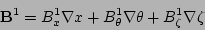
The derivation proceeds by writing the perturbed magnetic field
 in terms of both contravariant components
 and covariant components
 :
:
 |
(4) |
 |
(5) |
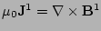
The perturbed current density  is written in terms of
contravariant components
is written in terms of
contravariant components
 |
(6) |
All perturbed variables are written as a series of Fourier
harmonics in the toroidal and poloidal angle-like variables,
and :
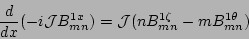
By linearizing the equilibrium equations, Eqs. (1),
(2) and (3), one obtains the equations
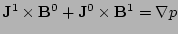 ,
,
 , and
, and
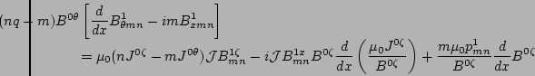
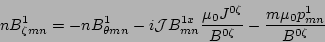
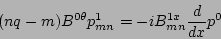
 . After some algebra, the following ordinary
differential equations are derived for the mix of contravariant
and covariant components of perturbed magnetic field, as well as
the perturbed pressure
. After some algebra, the following ordinary
differential equations are derived for the mix of contravariant
and covariant components of perturbed magnetic field, as well as
the perturbed pressure  [2]
[2]
 |
(7) |
 |
(8) |
 |
(9) |
 |
(10) |
In Hamada coordinates, the magnetic  is given by
 [4,7]. Equations
(7) and (8) form a pair of coupled ordinary
differential equations for each helical harmonic of the variable
[4,7]. Equations
(7) and (8) form a pair of coupled ordinary
differential equations for each helical harmonic of the variable
 . Equations
(9) and (10) can be used to eliminate
. Equations
(9) and (10) can be used to eliminate
 and . The perturbed covariant and
contravariant magnetic field components
and . The perturbed covariant and
contravariant magnetic field components  ,
,
 , and
, and  are determined from the algebraic
relations:
are determined from the algebraic
relations:
 |
(11) |
 |
(12) |
 |
(13) |
Equations (11), (12), and (13) are derived
by equating Eq. (4) and Eq. (5) and taking
the dot product with the gradients  ,
,  , and
, and
 .
The harmonic coupling implied by Eqs. (11)
through (13)
should be regarded as an upper bound estimate of the true
harmonic coupling, which can be substantially weakened by
differential rotation within the plasma.
.
The harmonic coupling implied by Eqs. (11)
through (13)
should be regarded as an upper bound estimate of the true
harmonic coupling, which can be substantially weakened by
differential rotation within the plasma.
The gradients of
 and, consequently, the
geometric terms in equations (11), (12), and
(13) can be determined from the shape of the equilibrium
flux surfaces in the following way: Suppose the shapes of the
equilibrium flux surfaces are given by the equations
and, consequently, the
geometric terms in equations (11), (12), and
(13) can be determined from the shape of the equilibrium
flux surfaces in the following way: Suppose the shapes of the
equilibrium flux surfaces are given by the equations
 |
(14) |
 |
(15) |
 |
(16) |
where the major radius  , the vertical position
  , and the
toroidal angle
, and the
toroidal angle  are given as functions of the Hamada
coordinates
. For axisymmetric equilibria, both
and are ignorable coordinates with period .
For any value of , the cross-sectional shape of the
corresponding flux surface is traced out by varying
between 0 and in Eqs. (14) and (15).
are given as functions of the Hamada
coordinates
. For axisymmetric equilibria, both
and are ignorable coordinates with period .
For any value of , the cross-sectional shape of the
corresponding flux surface is traced out by varying
between 0 and in Eqs. (14) and (15).
Then, from the gradients of Eqs. (14) through
(16)
 |
(17) |
 |
(18) |
 |
(19) |
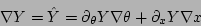
it follows that
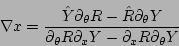 |
(20) |
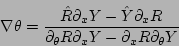 |
(21) |
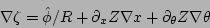 |
(22) |
and the Jacobian is given by
 . In these
equations,
. In these
equations,
 are unit vectors along
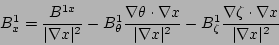
 . Application of the expressions for the gradients of
above in equations (11), (12),
and (13), leads to the following form for the mixing
equations:
. Application of the expressions for the gradients of
above in equations (11), (12),
and (13), leads to the following form for the mixing
equations:
![\begin{displaymath}[(\partial_{\theta}R)^{2} + (\partial_{\theta}Y)^{2}]B^{1\the...
...\theta} Y) + B^{1}_{\theta} +
B^{1}_{\zeta} \partial_{\theta}Z
\end{displaymath}](img60.png) |
(23) |
 |
(24) |
 |
(25) |
Eqs. (7 - 10) for the harmonics of  ,
,
 ,
,  , and
, and  together with Eqs.
(23 - 25) for the components ,
, and form a complete systems of
equations.
together with Eqs.
(23 - 25) for the components ,
, and form a complete systems of
equations.
Next: Width of a Magnetic
Up: Quasi-linear Tearing Mode Equations
Previous: Quasi-linear Tearing Mode Equations
transp_support
2008-12-08