Example 2 - contour plots

Example 2 - contour plots | 
|
To find out more about netCDF, see http://www.unidata.ucar.edu/packages/netcdf/
To run this example, you must download the following files:
gsun02n.ncland then type:
gsn_code.ncl
ncl < gsun02n.ncl
| Frame 1 | Frame 2 | Frame 3 | Frame 4 | Frame 5 |
|---|---|---|---|---|
| 
| 
| 
| 
|
(Click on any frame to see it enlarged.)
  1. load "gsn_code.ncl"
  2.
  3. begin
  4.
  5.   cdf_file = addfile("$NCARG_ROOT/lib/ncarg/data/cdf/contour.cdf","r")
  6.
  7.   temp = cdf_file->T(0,0,:,:)               ; temperature
  8.   Z    = cdf_file->Z(0,0,:,:)               ; geopotential height
  9.   pres = cdf_file->Psl(0,:,:)               ; pressure at mean sea level
 10.   lat  = cdf_file->lat                      ; latitude
 11.   lon  = cdf_file->lon                      ; longitude
 12.
 13.   temp = temp - 273.15                      ; Convert Kelvin -> Celsius
 14.   pres = pres * 0.01                        ; Convert Pa -> mb
 15.   temp@units = "(C)"                        ; Change units to reflect
 16.   pres@units = "(mb)"                       ; conversion done.
 17.
 18.   xwks = gsn_open_wks("x11","gsun02n")      ; Open an X11 workstation.
 19.
 20.   plot = gsn_contour(xwks,temp,False)       ; Draw a contour plot.
 21.
 22. ;----------- Begin second plot -----------------------------------------
 23.
 24.   resources                 = True       ; Indicate you want to set some
 25.                                          ; resources.
 26.
 27.   resources@cnMonoLineColor = False      ; Turn off the drawing of
 28.                                          ; contours lines in one color.
 29.
 30.   resources@tiMainString    = "Temperature (C)"  ; Create a title.
 31.
 32.   plot = gsn_contour(xwks,temp,resources)  ; Draw a contour plot.
 33.
 34. ;----------- Begin third plot -----------------------------------------
 35.
 36.   resources@cnFillOn          = True        ; Turn on contour line fill.
 37.   resources@cnMonoFillPattern = False       ; Turn off using a single fill
 38.                                             ; pattern.
 39.   resources@cnMonoFillColor   = True
 40.   resources@cnMonoLineColor   = True
 41.
 42.   resources@tiXAxisString    = lon@long_name
 43.   resources@tiYAxisString    = lat@long_name
 44.   resources@sfXArray         = lon
 45.   resources@sfYArray         = lat
 46.
 47.   plot = gsn_contour(xwks,temp,resources)   ; Draw a contour plot.
 48.
 49. ;---------- Begin fourth plot ------------------------------------------
 50.
 51.   resources@cnMonoFillPattern     = True     ; Turn solid fill back on.
 52.   resources@cnMonoFillColor       = False    ; Use multiple colors.
 53.   resources@cnLineLabelsOn        = False    ; Turn off line labels.
 54.   resources@cnInfoLabelOn         = False    ; Turn off informational
 55.                                              ; label.
 56.   resources@cnLinesOn             = False    ; Turn off contour lines.
 57.
 58.   resources@pmLabelBarDisplayMode = "Always" ; Turn on label bar.
 59.   resources@lbPerimOn             = False    ; Turn off perimeter on
 60.                                              ; label bar.
 61.
 62.   resources@tiMainString    = Z@long_name
 63.   resources@tiMainFont      = 26
 64.   resources@tiXAxisFont     = 26
 65.   resources@tiYAxisFont     = 26
 66.
 67.   plot = gsn_contour(xwks,Z,resources)    ; Draw a contour plot.
 68.
 69. ;---------- Begin fifth plot ------------------------------------------
 70.
 71.   cmap = (/(/0.,0.,0./),(/1.,1.,1./),(/.1,.1,.1/),(/.15,.15,.15/),\
 72.          (/.2,.2,.2/),(/.25,.25,.25/),(/.3,.3,.3/),(/.35,.35,.35/),\
 73.          (/.4,.4,.4/),(/.45,.45,.45/),(/.5,.5,.5/),(/.55,.55,.55/),\
 74.          (/.6,.6,.6/),(/.65,.65,.65/),(/.7,.7,.7/),(/.75,.75,.75/),\
 75.          (/.8,.8,.8/),(/.85,.85,.85/)/)
 76.
 77.   gsn_define_colormap(xwks,cmap)          ; Define a new color map.
 78.
 79.   resources@tiMainString    = pres@long_name
 80.
 81.   plot = gsn_contour(xwks,pres,resources) ; Draw a contour plot.
 82.
 83.   print(temp(2:5,7:9))             ; Print subset of "temp" variable.
 84.
 85.   print(temp!0)                    ; Print the dimension names for the
 86.   print(temp!1)                    ; first two dimensions of T.
 87.   print(temp@long_name)            ; Print "long_name" and "units"
 88.   print(temp@units)                ; attributes of "T".
 89.   print(temp&lat)                  ; Print coordinate variables "lat"
 90.   print(temp&lon)                  ; and "lon".
 91.
 92.   ascii_file = "data.asc"                 ; Create name of ASCII file.
 93.   system("/bin/rm -f " + ascii_file)      ; Remove ASCII file.
 94.   asciiwrite(ascii_file,temp(7:3:2,0:4))  ; Write part of temp to ASCII
 95.                                           ; file.
 96.   delete(plot)       ; Clean up.
 97.   delete(temp)
 98.   delete(resources)
 99. end
load "gsn_code.ncl"
Load the NCL script that contains the functions and procedures (the ones that start with "gsn_") that are used in this example. load in NCL works much like include works in C and Fortran 90 programs.
begin
Begin the NCL script.
cdf_file = addfile("$NCARG_ROOT/lib/ncarg/data/cdf/contour.cdf","r")
Open a netCDF file with addfile, a
function for providing a reference to many of the data formats that
NCL supports. For a list of these data formats, see the "File input and
output" section of the chapter "Introduction."The first argument of addfile (a string) is the file name, and the file type is determined by its suffix. In this case, the suffix ".cdf" indicates that it is a netCDF file. A suffix of ".nc" would have also worked.
Important note: The actual file name does not need to contain this suffix; it is needed just for NCL to know what kind of file it is dealing with. If the file name with the suffix doesn't exist in the directory that you specify, then NCL looks for the file without the suffix. For example, if the actual file is called "x" and it's a netCDF file, you would pass "x.nc" to addfile and NCL would look for both "x.nc" and "x".
The second argument to addfile is a string indicating whether you are reading ("r"), writing ("w"), or creating ("c") the file.
Another important note: This function does not read in any data from the netCDF file; it only returns a reference to the file.
  temp = cdf_file->T(0,0,:,:)
  Z    = cdf_file->Z(0,0,:,:)
  pres = cdf_file->Psl(0,:,:)
  lat  = cdf_file->lat
  lon  = cdf_file->lon
Now that you have a reference to the netCDF file you just opened, you can access all the variables and other information stored in it. T, Z, Psl, lat, and lon are all variables in the netCDF file. T and Z both have four dimensions corresponding to time, level, latitude and longitude, and Psl has three dimensions corresponding to time, latitude, and longitude. Remember, NCL uses "C" type indexing: the first element is index 0, and the fastest varying dimension is the rightmost dimension.
The syntax "->" is used to access variables within a file opened by addfile. You can select subsets of an array by using a colon to indicate the range to select. For more information on array processing and selection, see the "Array processing" section of the "Introduction" chapter.
The syntax "(0,0,:,:)" is used to select the first time step and the first level of variables T and Z in the netCDF file, and the syntax "(0,:,:)" selects the first time step of variable Psl. These three netCDF variables are stored to local NCL variables temp, Z, and pres, respectively.
If you don't indicate any range of values, as is done with the lat and lat variables, then all the values are selected.
The above assignment statements also retains any metadata information that the netCDF variables may contain, like attributes, named dimensions, and coordinate variables (concepts discussed below).
  temp = temp - 273.15
  pres = pres * 0.01
Using NCL's array syntax, convert all the values in temp from Kelvin to Celsius, and the values in pres from Pascals to millibars. Because these variables were previously defined, they retain any existing attributes, dimension names and coordinate variables (concepts discussed below).
Lines 7 and 8 could have been combined with lines 13 and 14 above as follows:
  temp = cdf_file->T(0,0,:,:) - 273.15     ; Won't retain metadata
  pres = cdf_file->Psl(0,:,:) * 0.01       ; of T or Psl.
However, this approach won't retain any metadata information from the netCDF file. The only thing that would be carried over from the above two statements would be a missing value, if there is one (missing values are discussed below). You can read more about these value-only assignments in the "Value-only assignment" section of the "NCL variables overview."
  temp@units = "(C)"
  pres@units = "(mb)"
Since the units for temp and pres have changed, the above changes creates the "units" attribute (if the "units" attribute didn't exist previously) to reflect the new units. Note that setting this attribute doesn't have any effect on the NCL code, but it is good programming practice to update metadata information, and you may want to use this information later in a title or a label.
xwks = gsn_open_wks("x11","gsun02n")
Open an X11 workstation for which to draw the contour plots.
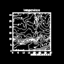
plot = gsn_contour(xwks,temp,False)Create and draw a contour plot of the 2-dimensional array temp. The first argument of the gsn_contour function is the workstation variable returned from the previous call to gsn_open_wks. The next argument is the 2-dimensional scalar field to be contoured, which can be of type float, double, or integer. The last argument is a logical value indicating whether you have set any resources. To get the default contour plot that NCL provides, pass the value False for the last argument.
The default contour plot drawn contains labeled tick marks and an "informational" label at the bottom right of the plot, indicating the range and spacing of the contour levels. Later examples show how to turn this informational label off, and how to customize the tick marks. Also, since no ranges have been defined for the X and Y axes in this plot, the range values default to 0 to n-1, where n is the number of points in that dimension.
If the variable being contoured has an attribute called "long_name", then gsn_contour uses this attribute as a title for the plot. In this case, temp does have a "long_name" attribute (the string "temperature"), so this is used to title the plot. If there is no "long_name" attribute, or if there is one defined but you don't want it for a title, then you can use the tiMainString resource to define your own title. An example is shown in the next plot.
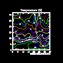
;----------- Begin second plot -----------------------------------------Draw the same contour plot, only this time draw the contour lines in color by setting some contour resources.
resources = TrueHere you are using resources to change the look of a plot (see example 1 for an explanation on how resources are set). Contour plot resources are part of the "ContourPlot" group and all start with the letters "cn". They are documented in the "ContourPlot resource descriptions" section of the NCAR Graphics 4.1 Reference Manual.
Data associated with a contour plot is called a "ScalarField." ScalarField resources start with "sf" and are documented in the "ScalarField resource descriptions" section of the NCAR Graphics 4.1 Reference Manual.
resources@cnMonoLineColor = FalseOccasionally you will see resource names with the word "Mono" in them. In this case, by setting cnMonoLineColor to False, you are telling NCL that you don't want to use a single color for all the contour lines, so it uses the "plural" resource cnLineColors to determine the line color for each line. If cnMonoLineColor had been set to True, then all contour lines would have been drawn in the same color determined by the "singular" resource cnLineColor.
The cnLineColors resource is an example of a resource that is set dynamically when you run the NCL script. NCL determines how many contour levels you have, then sets cnLineColors with enough color indices to color each line.
resources@tiMainString = "Temperature (C)"Create a title for the second plot (thus overriding the default title provided by the "long_name" attribute).
plot = gsn_contour(xwks,temp,resources)Draw a new contour plot using the resources you just set.
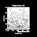
;----------- Begin third plot -----------------------------------------Draw the same contour plot, only this time fill the contours with the default hatching patterns. Also, explicitly define the ranges for the X and Y axes.
  resources@cnFillOn          = True
  resources@cnMonoFillPattern = False

  resources@cnMonoFillColor   = True
  resources@cnMonoLineColor   = True
By default, contour levels are not filled, so to get filled contours you need to set the resource cnFillOn to True. Also by default, when you fill contour levels, they are all filled in a solid color, so you need to set cnMonoFillPattern to False, telling NCL to use different fill patterns for each contour level.
A default set of fill patterns is provided dynamically through the cnFillPatterns resource. There are 17 different fill patterns available, each one represented by an integer from 1 to 17 (0 represents solid fill). So, to change the fill patterns, set the cnFillPatterns resource to an integer array with the same number of elements as you have contour levels.
You can see all the available fill patterns in the "Fill patterns" section of the NCAR Graphics 4.1 Reference Manual. By setting cnMonoFillColor and cnMonoLineColor both to True, you are telling NCL to use the same color for all the fills and lines (the default is the foreground color).
  resources@tiXAxisString    = lon@long_name
  resources@tiYAxisString    = lat@long_name
Create labels for the X and Y axes in the contour plot, using the attribute long_name defined for both lat and lon. The long_name attributes were inherited from the netCDF file when you read the lat/lon variables to local variables.
  resources@sfXArray         = lon
  resources@sfYArray         = lat
By setting the ScalarField resources sfXArray and sfYArray to the 1-dimensional arrays lon and lat, you can explicitly define the range for the X and Y axes.
plot = gsn_contour(xwks,temp,resources)Draw the contour plot. Note the new ranges for the X and Y axes, and the new title and X/Y axis labels.
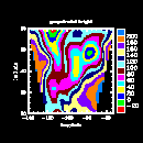
;---------- Begin fourth plot ------------------------------------------Draw a contour plot of the Z variable, fill the contour lines in solid colors and add a label bar on the side.
  resources@cnMonoFillPattern     = True
  resources@cnMonoFillColor       = False
  resources@cnLineLabelsOn        = False
  resources@cnInfoLabelOn         = False

  resources@cnLinesOn             = False
To fill the contours with solid fill in different colors, you need to set cnMonoFillPattern back to True, telling gsn_contour to use solid fills for all contour levels, and cnMonoFillColor to False to get multiple fill colors. The other resources turn off the labeling and drawing of contour lines, and the "informational" label you saw at the lower right corner in the previous contour plots.
  resources@pmLabelBarDisplayMode = "Always"
  resources@lbPerimOn             = False
There are times when you want to add other graphical objects to a plot, like a label bar, a legend, tick marks, or a title. In NCL, there's something called a "PlotManager" that lets you do this. It's called this because it "manages" the look of these additional objects and tries to make intelligent guesses about where the additional objects should be drawn with respect to the original plot. Also, if you resize the original plot, then these extra objects get resized as well. Some of these objects are always drawn by default, like tick marks and a title (if you specify one). A label bar is not drawn by default, so you need to tell the PlotManager to draw it by setting the PlotManager resource pmLabelBarDisplayMode to the predefined string "Always" (the default is "Never"). PlotManager resources start with "pm", and label bar resources start with "lb". These resources are documented in the "Labelbar resource descriptions" and "PlotManager resource descriptions" sections of the NCAR Graphics 4.1 Reference Manual.
As noted in example 1, predefined strings are case-insensitive, so the pmLabelBarDisplayMode resource could have also been set using "always" or "ALWAYS" or any another combination of uppercase and lowercase characters.
Setting the lbPerimOn resource to False indicates that you don't want a perimeter drawn around the label bar.
  resources@tiMainString    = Z@long_name
  resources@tiMainFont      = 26
  resources@tiXAxisFont     = 26
  resources@tiYAxisFont     = 26
Set the main title using the long_name attribute of Z. Also change the fonts of the title and the X and Y axis labels. A table of all the available fonts with their index values appears in the "Font table" section of the NCAR Graphics 4.1 Reference Manual. In this case, you are changing the font to "Times-bold."
Note: You could have also set this resource using the actual name of the font, "Times-bold", instead of the number 26.
plot = gsn_contour(xwks,Z,resources)Draw the fourth contour plot with a new dataset. Note that there are some areas in the contour plot that aren't being drawn. This is due to the presence of missing values in the data. By default, if the data being passed to any of the gsn_* plotting routines contains the attribute "_FillValue," then the value of this attribute is assumed to represent a missing value, and the gsn_* routines do not plot any data equal to this value. Missing values are covered in more detail in later examples, and you can also read about them in the "NCL variables overview" section of the NCL Reference Manual.
;---------- Begin fifth plot ------------------------------------------Draw a contour plot of the pres variable and fill the contour lines in solid colors using a grayscale color map that you define yourself.
  cmap = (/(/0.,0.,0./),(/1.,1.,1./),(/.1,.1,.1/),(/.15,.15,.15/),\
         (/.2,.2,.2/),(/.25,.25,.25/),(/.3,.3,.3/),(/.35,.35,.35/),\
         (/.4,.4,.4/),(/.45,.45,.45/),(/.5,.5,.5/),(/.55,.55,.55/),\
         (/.6,.6,.6/),(/.65,.65,.65/),(/.7,.7,.7/),(/.75,.75,.75/),\
         (/.8,.8,.8/),(/.85,.85,.85/)/)
For this plot, use grayscale values to fill the contour levels. To do
this, you need to define your own color map. Color maps are
represented by arrays of red, green, and blue float values
(referred to as RGB values)
ranging from 0. to 1. (to indicate the intensity of that particular
color). The first entry in a color map is the background color, and
the second entry is the foreground color. To get a color map of
grayscale values, use equal values for R, G, and B.For more information on creating your own color map, see the section "Color maps" in the "Basics" chapter.
gsn_define_colormap(xwks,cmap)To define a color map, use the NCL procedure gsn_define_colormap. The first argument is the workstation variable returned from a previous call to gsn_open_wks. The second argument is the color map you just created in lines 71-75.
  resources@tiMainString    = pres@long_name

  plot = gsn_contour(xwks,pres,resources)
Change the title to reflect the new data you are contouring, and draw a contour plot of the pres variable.
print(temp(2:5,7:9))Print a subset of temp (for each element 2 through 5 in the first dimension, print elements 7 through 9 in the second dimension). The print procedure takes as an argument any NCL variable and prints it out.
Please note that print does not do formatted printing of any kind. To get formatted printing, create one of your own using C or Fortran, and then write an NCL wrapper that allows you to call this routine from NCL. For more information on how to create wrappers for your C or Fortran subroutines, see the section "Incorporating your own Fortran or C code"" in the "Beyond the basics" chapter.
  print(temp!0)
  print(temp!1)
  print(temp@long_name)
  print(temp@units)
  print(temp&lat)
  print(temp&lon)
As noted in example 1, an NCL variable can contain additional information about itself called "metadata." Metadata is made up of attributes, coordinate variables, and named dimensions. The six print statements above print some of the metadata information of the temp variable that was passed on to it from the netCDF file. The "temp!0" syntax references the dimension name of the first dimension, temp&lat references the coordinate variable called lat, and temp@long_name references the attribute called "long_name". If any of this metadata does not exist, then the print statement issues an error message.
For more information on attributes, coordinate variables, and named dimensions in NCL, see the "Variables" section in the chapter "Introduction."
  ascii_file = "data.asc"
  system("/bin/rm -f " + ascii_file)
  asciiwrite(ascii_file,temp(7:3:2,0:4))
Write a subset of the temperature data to an ASCII file using asciiwrite. The
first argument of asciiwrite is the file name to which the
data will be written, and the second argument is the data to
write. The syntax "7:3:2" selects indices 7 to 3 with a
stride of 2, so only indices "7", "5", and "3" are selected for the
first dimension (in that order).The system call takes a string as an argument and executes a UNIX system command from NCL. In this case, it is being used to remove the file before writing to it. The "+" symbol, in addition to being used as an arithmetic operator, is also used in NCL to concatenate strings.
For more information on asciiwrite, system, and other NCL functions and procedures, see the "Built-in NCL functions and procedures" section of the NCL Reference Manual.
  delete(plot)
  delete(temp)
  delete(resources)
Clean up by deleting some variables you don't need anymore. As stated in the previous example, this is not really necessary since you are about to end the NCL script, but removing variables you don't need is a good habit to get into.
end
End the NCL script.