"""
Example -- Direct Comparison of Data with IPEC Modeling
=======================================================
This script compares the IPEC model plasma response to experimental data.
These shots where taken from J. King's 2013-23-01 experiment validating
3D magnetics response models.
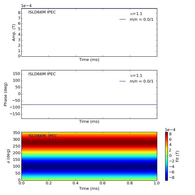
The scrip contains a 1 to 1 comparison between midplane saddle loop
experimental and modeled signals. Modeled signals are calculated
by interpolating single mode responses from an r,z grid to many points
across the sensor's surface and then taking the appropriate average.
A recomended excersise is to compare vacuum pickup. For the model, this
simply means using cbrzphi in place of pbrzphi. For the experiment,
vacuum picjup for each sensor can be obtained by subtracting the compensated
data from the original data.
"""
# standard modules
import numpy as np
# local modules
import magnetics
plt = magnetics.plt
############################################## Variables
shot = 153485
time = 3795
barray = magnetics.differenced_arrays['ISLD66M']
brzphi, = magnetics.model.read('g153485.{:05}.00096_100_ipec_brzphi_n1.out'.format(time)) # total perturbed b
cbrzphi, = magnetics.model.read('g153485.{:05}.00096_100_ipec_cbrzphi_n1.out'.format(time)) # vacuum perturbed b
pbrzphi = brzphi-cbrzphi # plasma perturbed b
############################################## 1 to 1 Comparisons
# get synthetic signals
array_ipec = barray.deepcopy()
array_ipec.set_model(brzphi)
# get measured plasma resp.
array_data = barray.deepcopy()
array_data.set_data(shot)
array_comp = array_data.compensate(fun_type='transfer',il=True,iu=True,c=False,
xlim=(time-100,time+100),pair=True)
array_comp = array_comp.smooth(5)
array_comp = array_comp.remove_baseline(time-100,time+100,False)
# get position,signal by hand
x,model,signal = [],[],[]
for key in array_ipec.sensors:
x.append(array_ipec.sensors[key].center[2])
model.append(array_ipec.sensors[key].y[0]) # no time dependence
signal.append(array_comp.sensors[key].newx([[time,]]).y[0]) # interpolte to time
x,model,signal =np.array(zip(*sorted(zip(x,model,signal))))
x = x *180/np.pi
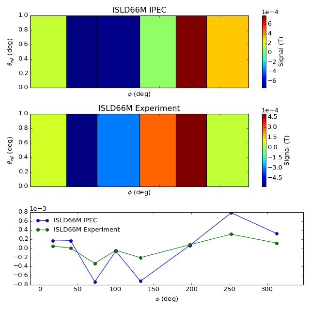
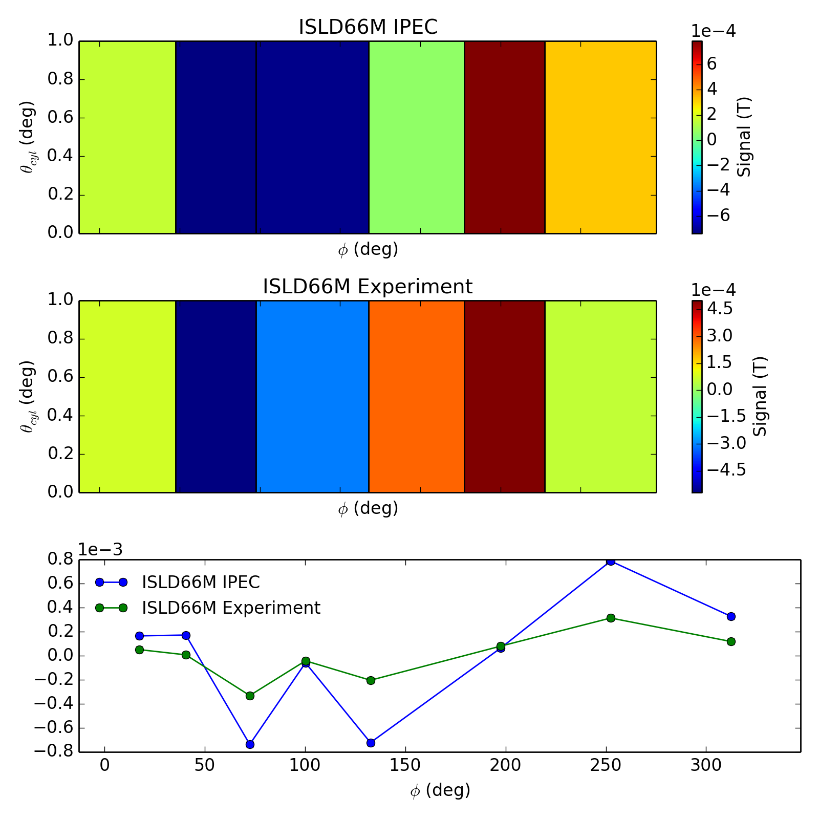
# plot
f,axes = plt.subplots(3,figsize=(8,8))
f = array_ipec.plotprobes(dim=2,time=0.5,axes=axes[0])
axes[0].get_legend().set_visible(False)
axes[0].set_title(barray.name+' IPEC')
f = array_comp.plotprobes(dim=2,time=0.5,axes=axes[1])
axes[1].get_legend().set_visible(False)
axes[1].set_title(barray.name+' Experiment')
axes[2].plot(x,model ,marker='o',label=barray.name+' IPEC')
axes[2].plot(x,signal,marker='o',label=barray.name+' Experiment')
axes[2].legend()
axes[2].set_xlabel(r'$\phi$ (deg)')
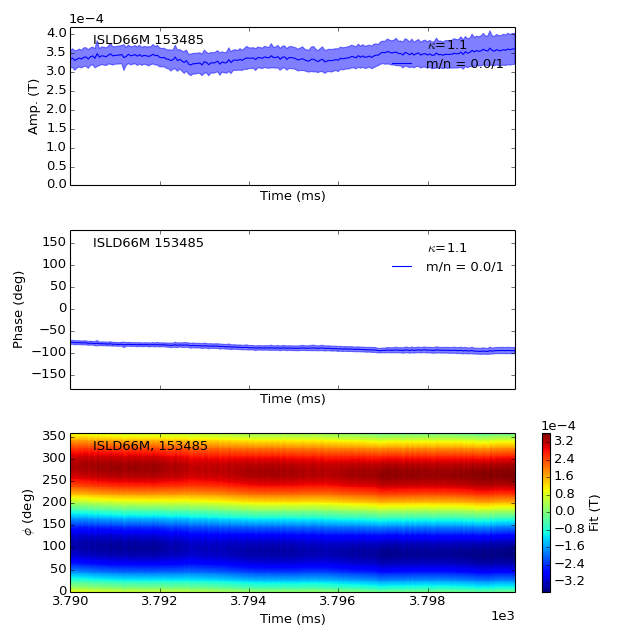
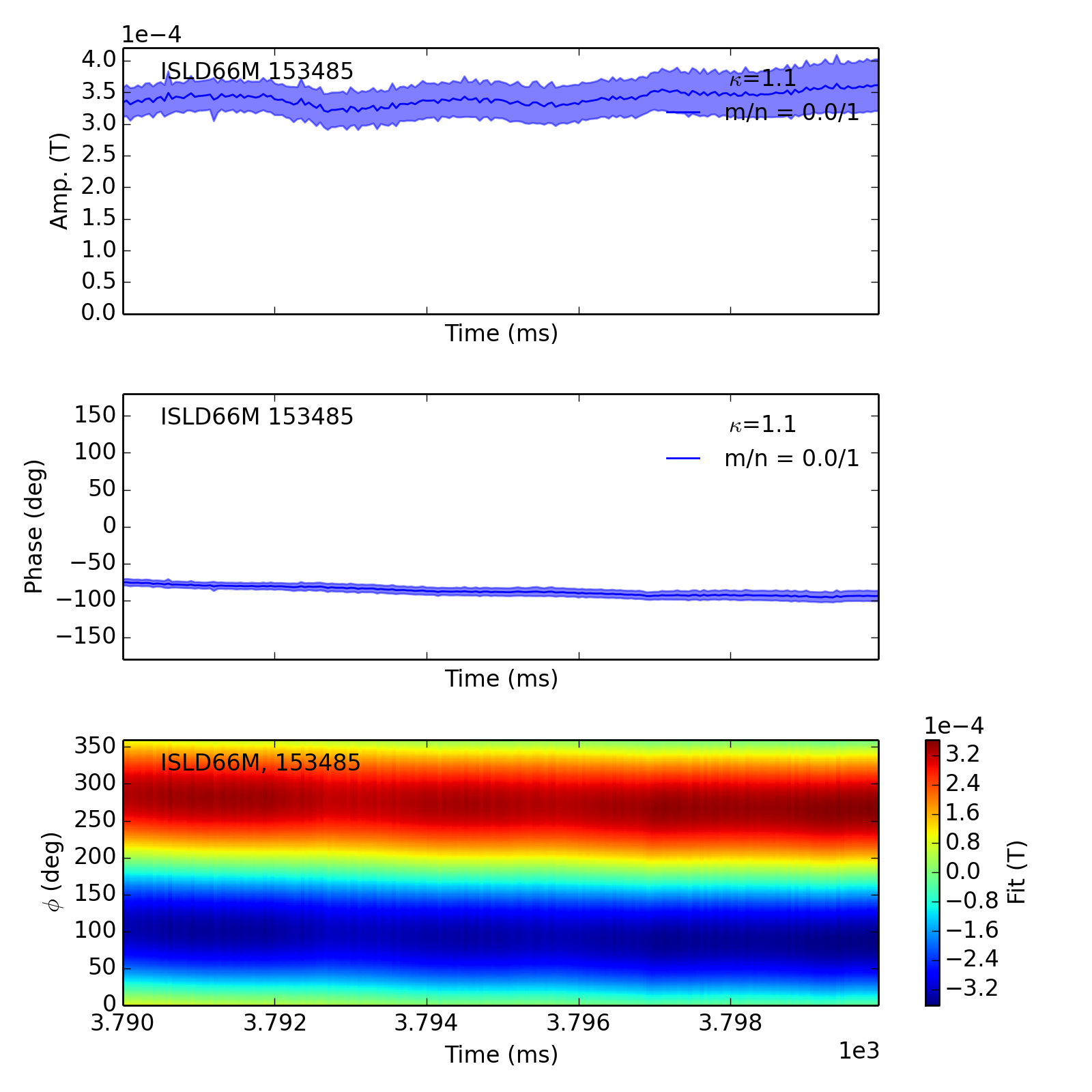
############################################## Synthetic Mode Fitting
array_comp.fit.update(ns=[1],ms=[0],xlim=(time-5,time+5))
array_comp.fit.plot()
array_ipec.fit.update(ns=[1],ms=[0])
array_ipec.fit.plot()
plt.show()
