This is the main module of the pyMagnetics pakcage. Its purpose is toprovide tools for retrieving, manipulating, and visualizing DIII-D magnetics data.
The module is dependent on almost all of the other modules in the package, and thus includes to dependence on Tom’ Osborn’s pyD3D package data module.
When automating array manipulation, please keep the following notes in mind:
The most basic element of this module is the Sensor object. These objects have data retrieval, geometric visualization, and data visualization method built into them. However, it is often burdensom to handle many Sensors in parallel. The Array objects consist of multiple Sensors, neatly organized and with the Sensor methods mentioned above nicely streamlines for your convinience.
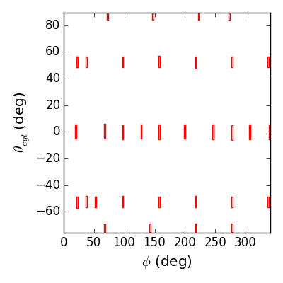
Lets look at a large array, consisting of all the mpid probes on the low field side:
>>> lfsbp = differenced_arrays['LFS MPIDs']
>>> f2d = lfsbp.plotprobes(dim=2,fill=False,color='r',legend=False)
>>> f2d.savefig(__packagedir__+'/doc/examples/magnetics_2darray.png')
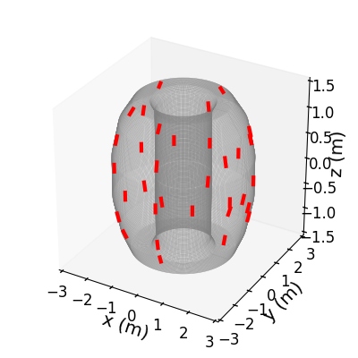
>>> f3d = lfsbp.plotprobes(dim=3,color='red')
>>> f3d = d3dgeometry.vessel.plot3d(wireframe=True,linewidth=0.1,color='grey',figure=f3d)
>>> f3d.savefig(__packagedir__+'/doc/examples/magnetics_3darray.png')
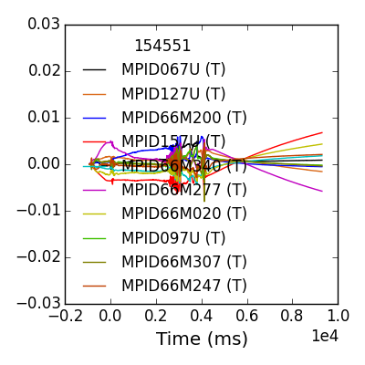
Now lets limit ourselves to a typical 1D array, and look at the raw data.
>>> mpidm = differenced_arrays['MPID66M']
>>> success = mpidm.set_data(154551)
Calling set_data for sensors in MPID66M array.
>>> fdata = mpidm.plotdata()
>>> fdata.savefig(__packagedir__+'/doc/examples/magnetics_data.png')
For large arrays, displaying all the data can be ugly and slow, try out the search keyword (search=‘200’ for example) on your own.
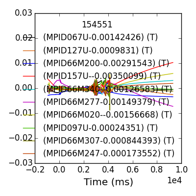
One thing we immediately see is that each sensor has a unique evolution in early time, which often dominates the amplitude in time. This is due to toroidal field and the forming poloidal field during the startup and Ip ramp. We do not trust this as a true 3D signal. A common way of removing the pickup from our studies of later times is to baseline before the time of interest.
>>> mpidm = mpidm.remove_baseline(2900,2930,slope=False)
Calling remove_baseline for sensors in MPID66M array.
>>> fdata = mpidm.plotdata()
>>> fdata.savefig(__packagedir__+'/doc/examples/magnetics_data_baselined.png')
The array object comes with an ossociated ‘fit’ method, which in our 1D example reproduces simple toroidal sinusoid amplitude-phase fitting.
>>> fit = mpidm.fit(ns=[1],ms=[0],xlim=(2900,3000))
SVD found 2 coherent structures of interest
Fitting structure 1
Raw rank, condition number = 2, 1.42
Eff rank, condition number = 2, 1.42
Fitting structure 2
Raw rank, condition number = 2, 1.42
Eff rank, condition number = 2, 1.42
Notice that the fitting method performs an SVD on the data matrix (PxT where P is the number of probes and T is the number of time points) and finds 2 coherent structures. The coherency metric includes eigenmodes progressively until the cumalitive energy is above 98% of the total. In our case, the modes can be understood as like to the sine and cosine components of the rotating n=1 mode. Each mode structure is individually fit to the spacial basis functions corresponding to the specified modes and geometry and then combined in time using the right singular vectors of the data matrix.
The energy and singular vectors can be viewed using built in methods.
>>> fsvde = fit.svd_data.plot_energy(cumulative=True)
>>> fsvde.savefig(__packagedir__+'/doc/examples/magnetics_svd_data_energy.png')
>>> fsvdt = fit.svd_data.plot_vectors(side='right')
>>> fsvdt.savefig(__packagedir__+'/doc/examples/magnetics_svd_data_time.png')

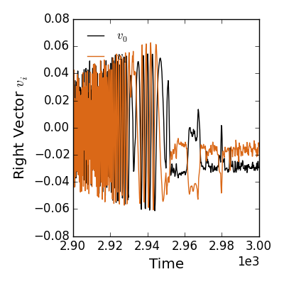
There is a lot of power in these quantities. There is physics understanding to be gained by isolating distinct coherent structures and their unique time behaviors. From a more practicle standpoint, the energy cut-off reduces the incoherent noise fed into our find spacial fits. Ultimately, however, we want to see the final fit to our basis functions in space and time.
No problem!
>>> fbasic = fit.plot()
Plotting fit for n = 1
>>> fbasic[0].savefig(__packagedir__+'/doc/examples/magnetics_1dfit.png')
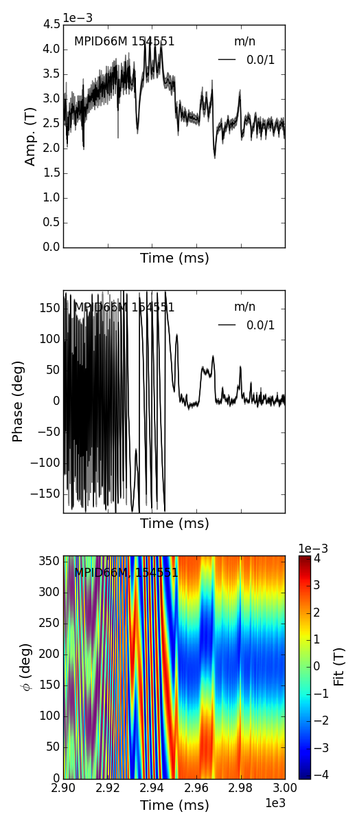
Notice the error in the amplitude and phase of the fit is shown graphically throughout time. The fit plotting function can return multiple plots, lets take a more complicated example to see why.
The magnetics module was made to handle 2D fits as naturally as in th 1D case.
>>> success = lfsbp.set_data(154551)
Calling set_data for sensors in LFS MPIDs array.
>>> lfsbp = lfsbp.remove_baseline(2900,2930)
Calling remove_baseline for sensors in LFS MPIDs array.
>>> fit = lfsbp.fit(ns=[1],ms=np.arange(-8,0),xlim=(2900,3000))
SVD found 4 coherent structures of interest
Fitting structure 1
Raw rank, condition number = 16, 7.65e+04
Eff rank, condition number = 10, 10
Fitting structure 2
Raw rank, condition number = 16, 7.65e+04
Eff rank, condition number = 10, 10
Fitting structure 3
Raw rank, condition number = 16, 7.65e+04
Eff rank, condition number = 10, 10
Fitting structure 4
Raw rank, condition number = 16, 7.65e+04
Eff rank, condition number = 10, 10
>>> f2d = fit.plot(dim=0)
Plotting fit for n = 1
>>> f3d = fit.plot(dim=3,time=2940)
Scroll over axes to change time
>>> f2d[0].savefig(__packagedir__+'/doc/examples/magnetics_2dfit1.png')
>>> f3d[0].savefig(__packagedir__+'/doc/examples/magnetics_2dfit2.png')
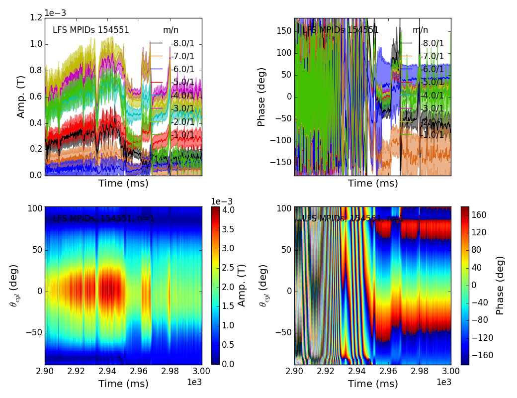
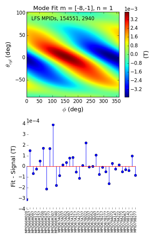
That is it! These are the Mode Fits.
These plots are highly interactive. In your ipython session, move the mouse over one of the axes in the second figure and scroll to show the mode evolving in time (spinning, locking, etc.). Try plotting with dim=-2, and watching the amplitude evolve.
If you want the actual fit parameters, the (n,m) mode numbers and the complex amplitude for each pair can be accessed using the nms and anm attributes. The b_n method gives the amplitude of a single toroidal mode number as a function of the poloidal variable, and interp2d gives the total fit on the 2D space.
Finally, you may be wondering what the ranl and condition numbers printed for each structure are. These are the rank and condition number of the basis function matrix A used to fit the mode amplitudes x by solving Ax = b where b is array of sensor signals for the structure. A second and completely independent SVD is done on the basis matrix A, and the singular values below a certain condition number (a key word argument of the fit), they are removed. To see the singular values, right and left singular vectors of this SVD use the methods of the fit.svd_basis instancce. To visualize the eigenmodes of this basis matrix in real space, use the fitvector key word in the usual plot method.
Lets look at some of the first complex modes in the eigen-space for the LFS MPIDs. The first 5 correspond to the 10 cos,sin modes used in our fit with effective rank 10. The higher ones correspond to combination of cos,sin modes that we deamed insufficiently constrrained to be used in our analysis.
>>> f,ax = plt.subplots(4,2,figsize=plt.rcp_size*[3,4])
>>> for i,a in enumerate(ax.ravel()):
...    f = fit.plot(dim=3,axes=a,fitvector=i+1)[0]
...    t = a.set_title('R-Sing. Vector {:}'.format(i+1))
...    f = lfsbp.plot2d(color='k',fill=False,axes=a)
Scroll over axes to change time
Calling plot2d for sensors in LFS MPIDs array.
Scroll over axes to change time
Calling plot2d for sensors in LFS MPIDs array.
Scroll over axes to change time
Calling plot2d for sensors in LFS MPIDs array.
Scroll over axes to change time
Calling plot2d for sensors in LFS MPIDs array.
Scroll over axes to change time
Calling plot2d for sensors in LFS MPIDs array.
Scroll over axes to change time
Calling plot2d for sensors in LFS MPIDs array.
Scroll over axes to change time
Calling plot2d for sensors in LFS MPIDs array.
Scroll over axes to change time
Calling plot2d for sensors in LFS MPIDs array.
>>> f.savefig(__packagedir__+'/doc/examples/magnetics_basis_functions_2d.png')
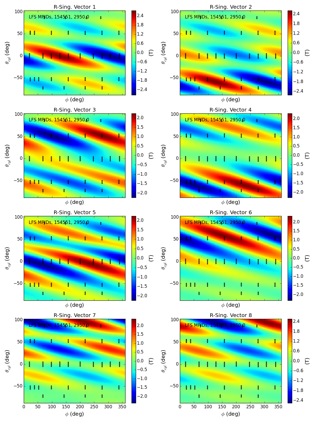
Thats awsome! We can see how the first eigen-modes are consentrated in the areas with many sensors, and thus well constrained by the measurements. As the mode number increases the regions of large amplitude migrate to areas between sensors, and the modes excluded by the conditioning are obviously combinations of cos,sin modes that the sensors can barely see.
Bases: pyMagnetics.magdata.Data, object
2d surface magnetic sensors object with built in data retrieval, model retrieval, and visualization.
# RETURNS A NEW DATA CLASS INSTANCE
cdfput( self, # Write Data instance to netcdf file name = None, # File name, if none use self.yname path=’.’, # Directory path to file tfile = None, # If not None, add cdf file to this tarfile instance and delete original cdf file format = ‘NETCDF4’,
- # Form of netCDF file
- # netCDF files come in several flavors (‘NETCDF3_CLASSIC’, # ‘NETCDF3_64BIT’, ‘NETCDF4_CLASSIC’, and ‘NETCDF4’). The first two flavors # are supported by version 3 of the netCDF library. ‘NETCDF4_CLASSIC’ # files use the version 4 disk format (HDF5), but do not use any features # not found in the version 3 API. They can be read by netCDF 3 clients # only if they have been relinked against the netCDF 4 library. They can # also be read by HDF5 clients. ‘NETCDF4’ files use the version 4 disk # format (HDF5) and use the new features of the version 4 API. The # ‘netCDF4’ module can read and write files in any of these formats. When
quiet = False, # IF True, DON’T PRINT FILE NAME WRITTEN TO )
Attempt to compensate sensor data for vacuum coupling to 3D coils using pcs point names for coil currents.
Additional kwargs passed to response_function.compensate.
compress( # REMOVE VALUES FROM self (IN PLACE) WHERE CONDITION IS NOT SATISFIED. # CONDITION MUST HAVE THE SAME LENGTH AS THE AXIS ALONG WHICH COMPRESSION IS DONE. # IF CONDITION IS ‘unique’ MAKES AXIS UNIQUE VALUES (I.E. NO TWO X VALUES ARE THE SAME. # THE INSTANCE IS SORTED ALONG axis. self, condition, # LOGICAL CONDITION WITH LENGTH OF axis OR ‘unique’ TO COMPRESS OUT
# VALUES WITH THE SAME x (FIRST VALUE IS TAKEN)
axis = 0, # AXIS ALONG WHICH YOU WANT TO COMPRESS, F NOTATION, I.E. axis=0 IS self.x[0] )
conj( # COMPLEX CONJUGATE self, ) # RETURNS NEW Data INSTANCE, z, WITH z.y = conj(self.y)
contour( # GENERATE SERIES OF CONTOUR LINES FOR 2-D DATA self, vc = None, # SEQUENCE OF CONTOUR VALUES nc = 10, # IF vc IS None THEN nc=NUMBER OF CONTOURS BETWEEN min(self.y) and max(self.y) zmax = None, # IF NOT None VALUES OF self.y ABOVE zmax ARE IGNORED IN CONTOURING ) # RETURNS A NEW Data INSTANCE z WITH # z.y[ i, 0, : ] = X0 VALUES FOR THE i’TH CONTOUR # z.y[ i, 1, : ] = X1 VALUES FOR THE i’TH CONTOUR # z.x = [ INDEX ALONG CONTOUR, X INDEX , CONTOUR INDEX ] # z.ncont[i] = NUMBER OF POINTS IN i’TH CONTOUR # z.kcont[i] = 10* INDEX OF VC FOR THE i’TH CONTOUR + IFLAG WHERE # IFLAG=0 FOR A CLOSED CONTOUR AND IFLAG=1 FOR AN OPEN CONTOUR
Returns copy.copy of Sensor object.
copy( # COPY ALL ATTRIBUTES OF A Data INSTANCE, RETUNS A NEW INSTANCE # WARNING ! copy.copy IS USED SO THAT IN MOST CASES NEW REFERENCES # ARE CREATED RATHER THAN COPIES, THUS ANY MUTABLE ATTRIBUTES CHANGED # IN THE COPIED INSTANCE WILL BE CHANGED IN THE ORIGINAL INSTANCE. THIS # IS AVOIDED IN THE CASE OF THE x AND xerror LISTS BY DOING FULL COPIES # (I.E. MAKING CHANGES TO x IN THE COPIED INSTANCE WILL NOT CHANGE THE # ORIGINAL). NOTE ALSO THAT THE ATTRIBUTE t_domains AND ANY HIDDEN # I.E. BEGENNING WITH _ ARE NOT COPIED. self, )
Returns copy.deepcopy of Sensor object.
der( # FIRST DERIVATIVE ALONG AXIS USING CENTRAL DIFFERENCE self, axis = 0, # X AXIS INDEX TO TAKE DERIVATIVE ALONG ) # RETURNS: NEW Data CLASS INSTANCE, z, A COPY OF self WITH # WITH z.y = DERIVATIVE, z.x[axis] = self.x[axis][1:-1]
First derivative along axis using central difference derivative( variable = 0, The index of the variable of the function with
respect to which the X{derivative} is taken
) Returns: New InterpolatingFunction Class instance with
values = Derivative and axes[variable] = axes[variable][1:-1]
dump( # DUMP Data INSTANCE X,Y DATA TO COLUMNS IN AN ASCII TEXT FILE. # WORKS WITH ANY NUMBER OF Y DIMENSIONS self, dfile = None, # Data name in file: IF None USE self.yname.
# If form == ‘REVIEW’ full file name = shot#dfile.dat # If form != ‘REVIEW’ full file name = dfile_shot#.dat or # dfile.dat if append_shot==False
form = None, # IF form.upper() == ‘REVIEW’ USE REVIEW DATA FILE NAME AND HEADLINES append_shot = True, # IF True AND form != ‘REVIEW’, SHOT NUMBER IN SUFFIX headline = True, # IF True AND form != ‘REVIEW’, WRITE A HEADLINE WITH COLUMN NAMES auxdat = True, # IF True, DUMP yaux DATA AS ADDITIONAL COLUMNS tfile = None, # IF NOT None, ADD DUMP FILE TO THIS tarfile INSTANCE AND DELETE ORIGINAL ASCII FILE quiet = False, # IF True, DON’T PRINT FILE NAME WRITTEN TO )
fft( # FAST FOURIER TRANSFORM USING FFTW # ONLY WORKS FOR FIXED X-AXIS SPACING, USE .newx FIRST # IF YOU HAVE VARIABLE SPACING self, axis = 0, # AXIS ALONG WHICH TO TAKE FFT xmin = None, # MINIMUM X VALUE TO INCLUDE xmax = None, # MAXIMUM X VALUE TO INCLUDE assume_real = True, # IF TRUE RETURNS REAL FFT (HALF THE NUMBER OF POINTS) detrend = True, # IF TRUE A LINEAR LEAST SQUARES FIT IS SUBTRACTED FROM
# DATA ARRAY BEFORE FFT IS PERFORMED
quiet = 1 # IF 0 PRINT OUT EXTRA INFO ) # RETURNS: NEW Data INSTANCE, z, z.y = fft(self.y), z.x = FREQUENCY (1/self.x)
Uses scipy.signal.firwin to design a spectral filter and then applies it to signal. Assumes 1D data. Overrides nyq, using the first time step in data.x[0] to calculate the nyquist frequency. All frequency cutoffs are thus in kHz, and must be between 0 and the nyquist frequency.
Suggested values : numtaps=40
Arguments and Key word arguments are taken from scipy.signal.firwin. Documentation below:
FIR filter design using the window method.
This function computes the coefficients of a finite impulse response filter. The filter will have linear phase; it will be Type I if numtaps is odd and Type II if numtaps is even.
Type II filters always have zero response at the Nyquist rate, so a ValueError exception is raised if firwin is called with numtaps even and having a passband whose right end is at the Nyquist rate.
Set to True to scale the coefficients so that the frequency response is exactly unity at a certain frequency. That frequency is either:
scipy.signal.firwin2
Low-pass from 0 to f:
>> from scipy import signal
>> signal.firwin(numtaps, f)
Use a specific window function:
>> signal.firwin(numtaps, f, window='nuttall')
High-pass (‘stop’ from 0 to f):
>> signal.firwin(numtaps, f, pass_zero=False)
Band-pass:
>> signal.firwin(numtaps, [f1, f2], pass_zero=False)
Band-stop:
>> signal.firwin(numtaps, [f1, f2])
Multi-band (passbands are [0, f1], [f2, f3] and [f4, 1]):
>> signal.firwin(numtaps, [f1, f2, f3, f4])
Multi-band (passbands are [f1, f2] and [f3,f4]):
>> signal.firwin(numtaps, [f1, f2, f3, f4], pass_zero=False)
fit( # FIT TO A USER DEFINED OR STANDARD FUNCTION USING NONLINEAR LEAST SQUARES self, func_in, # FITTING FUNCTION DEFINED IN USER ROUTINE OR STRING TO SELECT FROM A PREDEFINED SET.
# IF DEFINED IN A USER ROUTINE ARGUMENTS MUST BE ( C, X, PARAM = NONE ) WHERE # C IS A SEQUENCE OF THE COEFFICIENTS TO BE FIT, # X IS A LIST OF MATRICIES WHERE, E.G. MATRIX 0 GIVES THE VALUE # OF self.x[0] AT ALL POINTS ON THE GRID WHERE self.y IS DEFINED (THESE # MATRICIES ARE SET UP AUTOMATICALLY WHEN .fit IS CALLED), # PARAM IS EXTRA PARAMETERS (ALLOWS ARTERING THE FUNCTION) # USER DEFINED FUNCTIONS CAN BE IN THE CALLING MODULE OR PUT IN A MODULE # CALLED extra_fit_functions.py WHICH IS AUTOMATICALLY IMPORTED ALLOWING # A STRING = FUNCTION NAME TO BE USED FOR func_in AS WITH OTHER PREDEFINED. # STANDARD PREDEFINED FUNCTIONS ARE ONE OF THE FOLLOWING, # (SEE data_fit_functions MODULE FOR MORE INFO) # POLY: 1-D POLYNOMIAL ON X[0], ORDER DETERMINED BY LEN(C0) # GAUSS:1-D GAUSSIAN ON X[0],C[0]EXP( (X-C[1])**2*C[2] ) # POWER:N-D POWER LAW; X[0]**C[0]*X[1]**C[1]...*C[N] # TSPLFUN:TENSIONED SPLINE # LINFUN:1-D TWO LINE FIT, C[0]=SYM,C[1]=PED,C[2]=SLOPEIN,C[3]=SLOPEOUT # TANH:1-D HYPERBOLIC TANGENT, C[0]=SYM,C[1]=WID,C[2]=PED,C[3]=OFF,C[4]=ALP # TANH_QUAD_QUAD:HYPERBOLIC TANGENT WITH QUADRATIC INNER AND OUTER EXTENSIONS # TANH_QUAD_LIN:HYPERBOLIC TANGENT WITH QUADRATIC INNER AND LINEAR OUTER EXTENSIONS # TANH_QUAD_CONST:HYPERBOLIC TANGENT WITH QUADRATIC INNER AND CONSTANT OUTER EXTENSIONS # TANH_0OUT: TANH WITH QUAD INNER AND 0 OUTER EXTENSIONS # TANH_MULTI:HYPERBOLIC TANGENT WITH INNER AND OUTER CONTROLLED ORDER CONTROLLED BY PARAM # TNH0:1-D HYPERBOLIC TANGENT, C[0]=SYM,C[1]=WID,C[2]=PED,C[3]=OFF,C[4]=ALP # TNH0_0OUT: TANH WITH LINEAR INNER AND 0 OUTER EXTENSIONS
c0, # STARTING VALUE FO FIT COEFFICIENTS param = None, # EXTRA PARAMETERS TO PASS TO FUNCTION.SHOULD BE NUMBER OR SEQUENCE OF NUMBERS
# THAT CAN BE CAST AS A NUMERIC ARRAY (FOR MDS+ STORAGE)
# PROBLEMS WITH WITH ord = FALSE FIND A SOLUTION WITH TRADITIONAL LEAST SQUARES MINIMUNIZATION # WITH WEIGHTS SET BY Y ERRORS ONLY USING scipy.optimize.leastsq WITH THE FOLLOWING PARAMETERS. # SEE scipy.optimize.leastsq DOCUMENTATION FOR MORE DETAILS ON THESE PARAMETERS ftol = 1.49012e-8, # CALC TERMINATION OCCURS WHEN BOTH THE ACTUAL AND PREDICTED RELATIVE
# REDUCTIONS IN THE SUM OF SQUARES ARE AT MOST ftol. THEREFORE, ftol MEASURES # THE RELATIVE ERROR DESIRED IN THE SUM OF SQUARES.
maxfev = 0, # THE CALC IS TERMINATED IF NUM OF CALLS TO func = maxfev, IF SET TO 0 USES 100*(len(c)+1) epsfcn = 0.0, # STEP FOR FORWARD-DIFFERENCE APPROX(IF DFUN=None), IF 0 DETERMINED BY MACHINE PRECISION factor = 100., # A PARAMETER DETERMINING THE INITIAL STEP BOUND 0.1<factor<100 diag = None, # A SEQUENCT OF len(c) USED AS SCALE FACTORS FOR c. CAN BE USED TO MAKE ALL c’s O(1).
# PROBLEMS ord = TRUE FIND A SOLUTION WITH ORTHOGONALDISTANCE REGRESSION # ALLOWING FOR ERRORS IN BOTH X AND Y USING scipy.optimize.odr WITH THE FOLLOWING PARAMETERS. # SEE scipy.optimize.odr DOCUMENTATION FOR MORE DETAILS ON THESE PARAMETERS sstol = None, # FLOAT SPECIFYING THE TOLERANCE FOR CONVERGENCE BASED ON THE RELATIVE
# CHANGE IN THE SUM-OF-SQUARES. THE DEFAULT VALUE IS EPS**(1/2) WHERE EPS # IS THE SMALLEST VALUE SUCH THAT 1 + EPS > 1 FOR DOUBLE PRECISION COMPUTATION ON THE MACHINE. # SSTOL MUST BE LESS THAN 1.
ndigit = None,# INTEGER SPECIFYING THE NUMBER OF RELIABLE DIGITS IN THE COMPUTATION OF THE FUNCTION. accept_questionable = False, # IF TRUE THEN ACCEPT CONVERGED BUT QUESTIONABLE RESULTS
) # RETURNS: A NEW Data INSTANCE WITH self.y REPLACED BY THE FITTED VALUES AND THE FOLLOWING EXTRA ATTRIBUTES # Additional attributes of z: # z.fit_coef = ARRAY OF FIT COEFFICIENTS # z.fit_coeferr = ARRAY OF ERRORS IN FIT COEFFICIENTS # z.fit_coefcov = COEFFICIENT COVARIANCE ARRAY, DIAGONAL IS coeferr**2 # z.fit_nu = NUMBER OF FITTING PARAMETERS # z.fit_chisq = CHISQ OF FIT # z.fit_ch2prob = PROBABILITY OF THIS CHISQ VALUE # z.fit_condnum = CONDITION NUMBER FOR FIT (AVAILABLE IN ODR ONLY) # z.fit_fjac = JACOBIAN (dy_i/d_coef_j) (AVAILABLE IN ODR ONLY) # z.yerror = ERROR BAR OF FIT = jac * coefcov * jac.T (AVAILABLE IN ODR ONLY) # z.fit_func = func_in # z.fit_param = FUNCTION CONTROL PARAMETERS (PARAM) (NOT INCLUDE IF PARAM=None) # z.__call__ (i.e. INSTANCE CAN BE CALLED AS A FUNCTION) z(x)= VALUE OF FIT AT X. # WITH MORE THAN ONE DIMENSION z(x0,x1,...). x VALUES CAN BE NUMBERS OR SEQUENCES. # RETURNED VALUE IS AN ARRAY WITH SHAPE = ( len(xn), len(xn-1), .. len(x0)), OR # A NUMBER IF ONLY ONE VALUE IS RETURNED. FOR z.nx=1: z() RETURNS ROOT NEAR LOCATION # OF min(abs(z.y)); z(x0,ider) RETURNS DERIVATIVE OF ORDER ider AT x0.
imag( # IMAGINARY PART self, ): # RETURNS NEW Data INSTANCE, z, WITH z.y = imag(self.y)
int( # INTEGRATE USING TRAPIZOID RULE self, axis = 0, # AXIS TO INTEGRATE ALONG ) # RETURNS A NEW Data INSTANCE, z, WITH z.y = integral(self.y)
Integrate using trapizoid rule int( variable = 0, The index of the variable of the function with
respect to which the X{derivative} is taken
) Returns: New InterpolatingFunction Class instance with values = Integral
interp_fun( # CREATE A CALL METHOD FOR THE INSTANCE WHICH IS AN INTERPOLATING # FUNCTION. THE INTERPOLATED VALUE IS RETURNED WHEN THE INSTANCE # IS CALLED AS A FUNCTION. ANY NUMBER OF DIMENSIONS IS SUPPORTED # FOR LINEAR INTERPOLATION. THE ORDER OF THE X VALUES IN MULTI # DIMENSIONS CORRESPONDS TO THE X INDEX (I.E. THE OPPOSITE OF THE # INDEX ORDER IN Y). self, func = None, # NAME OF INTERPOLTING FUNCTION TO USE.
# NOTE THAT interp_fun IS CALLED AUTOMATICALLY IN .spline() AND .fit() # SO YOU DON’T NEED TO CALL IT DIRECTLY IF YOU HAVE USED THESE METHODS. # None: LINEAR INTERPOLATION # ‘spline’: INTERPOLATING CUBIC SPLINE (ALLOWS DERIVATIVES) # other string or python function : ‘INTERPOLATE’ WITH FIT FUNCTION # EITHER THE NAME OF A STANDARD FIT FUNCTION OR THE ACTUAL DESIRED # FIT FUNCTION (SEE .fit() DOCUMENTATIONS ). NOTE THAT IN CONTRAST # TO THE FIT METHOD self.y IS NOT REPLACED BY THE FITTED VALUES SO # THAT THE ‘INTERPOLATED’ VALUE MAY NOT MATCH self.y AT THE SAME X.
c0 = None, # INITIAL COEFFICIENTS FOR .fit() WHEN DOING FIT THROUGH .interp_fun() param = None,# CONTROL PARAMETERS TO PASS TO FIT FUNCTION, (SEE .fit() DOCUMENTATION) default = 0.,# DEFAULT VALUE FOR LINEAR INTERPOLATION (OUTSIDE OF X RANGE) # # __call__ METHOD ARGUMENTS: self(args) # *args,# FOR self.nx == 1:
# IF len(args) == 0: # RETURN ROOT # FOR SPLINE INTERPOLATING FUNCTION ALL ROOTS IN X[0] RANGE ARE FOUND, # FOR OTHER FORMS ROOT NEAREST LOCATION WHERE abs(self.y) IS MINIMUM # IF len(args) == 1: # RETURNS VALUES AT LOCATION(S) args[0] (args[0] CAN BE A SEQUENCE OR NUMBER) # IF len(args) == 2 and args[1] >=0: # RETURNS DERIVATIVE OF ORDER args[1] AT LOCATION(S) args[0] # (args[0] CAN BE A SEQUENCE OR NUMBER) # IF len(args) == 3 AND args[1] == -1: # RETURNS DEFINITE INTEGERAL BETEEN args[0] and args[2] # (args[0],args[2] MUST BE NUMBERS) # FOR self.nx > 1: # x0, x1, x2, ... CORRESPONTING TO THE DIFFERENT X AXIS, # WHERE x CAN BE A NUMBER OR SEQUENCE. # RETURNS: AN ARRAY WITH SHAPE (len(xn), len(xn-1), ... len(x0)) # OR SINGLE NUMBER CORRESPONDING TO VALUES AT x0,x1,...
)
inv_fft( # INVERSE FAST FOURIER TRANSFORM USING FFTW. # ONLY WORKS FOR FIXED X-AXIS SPACING, USE .newx FIRST IF YOU HAVE VARIABLE SPACING. # IT IS ASSUMED THAT THE INPUT DATA IS A FULL FOURIER TRANSORM, # I.E. EXTENDING FROM FREQ = 0 TO THE NYQUIST FREQUENCY FOR ASSUME_REAL=’TRUE’ AND INCLUDING # THE NEGATIVE FREQUENCY DATA FOR POINTS ABOVE THE NYQUIST FREQUENCY. SLICING WITH XMIN # AND XMAX IS DONE ZEROING OUT THE DATA OUTSICE THE SLICE INTERVAL ( A BAND PASS FILTER). self, axis = 0, # AXIS ALONG WHICH TO TAKE FFT fmin = None, # MINIMUM f VALUE TO INCLUDE fmax = None, # MAXIMUM f VALUE TO INCLUDE assume_real = True, # IF TRUE ASSUME self IS A REAL FFT (HALF THE NUMBER OF POINTS)
# AND USE SYMMETRY PROPERTIES OF THE FFT OF A REAL ARRAY # TO CONSTRUCT THE FULL FFT BEFORE INVERTING
quiet = 1 # IF 0 PRINT OUT EXTRA INFO ) # RETURNS: NEW Data INSTANCE, z, z.y = inv_fft(self.y), z.x = TIME (1/self.x)
list( # LIST NAMES AND RANGES OF Data CLASS INSTANCE self, )
Returns natural logarithm of data.
..note: By including this, we enable the numpy function to be applied directly to a data object (i.e. np.log(density)).
mdsput( # # WRITE DATA INSTANCE TO MDS+ AS A SIGNAL NODE. # # IF THE INSTANCE HAS FIT OR SPLINE ATTRIBUTES :fitname AND :fitdoc ALONG WITH THE # OTHER FIT AND SPLINE ATTRIBUTES ARE ADDED AS SUBNODES. THESE ARE USED TO RECONSTRUCT # THE FIT OR SPLINE WHEN THE DATA IS READ FROM MDS+. # # ONE LAYER OF NUMERIC OR STRING SUBNODES IS ALLOWED, ANY NUMBER OF LAYERS OF Data # INSTANCE SUBNODES IS ALLOWED AND HANDELED BY RECURSION. Data TYPE SUBNODES CAN IN # TURN HAVE ONE LAYER OF NUMERIC OR STRING SUBNODES. # SUBNODES ARE NAMED AS ENTRY IN self.__dict__.keys, SUBNODES DO NOT HAVE TAGNAMES. # self, tree, # MDS+ TREE TO STORE DATA IN path = ‘’, # BRANCH OF MDS+ TREE (DIRECTORY PATH) name = None, # NAME TO USE FOR MAIN NODE, IF NONE THEN = self.yname shot = None, # SHOT NUMBER, IF NONE THEN = self.shot tagname = None, # IF NOT NONE ATTACH THIS MDS+ TAGNAME TO THE NODE create = 0, # 0: IF NODE EXISTS AND IS OF CORRECT TYPE TRY TO WRITE TO IT,
# IF NO EXISTING NODE OR INCORRECT TYPE CREATE IT # 1: CREATE NEW NODE, DELETE OLD ONE IF IT EXISTS
comment = None, # COMMENT TO ADD AS SUBNODE open_tree = 1, # OPEN TREE ON CALL AND CLOSE ON RETURN,
# SET TO 0 FOR MULTIPLE WRITES TO SAME TREE
quiet = 0, # 1: PRINT EXTRA STUFF )
newx( # CREATE A NEW X AXIS BY LINEAR INTERPOLATION self, xnew = None, # IF xnew IS None: USE MIN DX FOR NEW SPACING ALONG EACH AXIS
# IF self.nx == 1: # IF xnew = NUMBER USE DX = xnew FOR SPACING OF NEW AXIS # IF xnew = ARRAY USE THIS FOR THE NEW AXIS # IF self.nx > 1: # IF xnew != None xnew MUST BE A LIST WITH VALUES OR None FOR EACH AXIS # IF xnew[i] IS None: USE MIN DX[i] FOR NEW SPACING ALONG I’TH AXIS # IF xnew[i] = NUMBER != 0 USE DX[i] = xnew[i] FOR SPACING OF NEW AXIS # IF xnew[i] = 0, no CHANGE ON THIS AXIS # IF xnew[i] = ARRAY USE THIS FOR THE NEW AXIS # # NOTE: CHANGING AXIS FOR self.nx > 1 CAN BE TIME CONSUMING SINCE INTERPOLATION # IS DONE FOR ALL POINTS, I.E. len(xnew[0])*len(xnew[1])*...
) # Returns: new Data instance on xnew
newy( # CREATE A NEW INSTANCE BASED ON THE CALLBACK FUNCTION ASSOCIATED WITH self. # EITHER VALUES OR DERIVATIVES CAN BE RETURNED. # IF self HAS NO CALLBACK FUNCTION AN INTERPOLATING SPLINE IS SET UP self, *args # args[0:self.nx]: args[i] IS AN ARRAY OF THE iTH X VALUES. IF = NONE USE self.x[i]
# args[self.nx,2*self.nx] : DERIVATIVE ORDER FOR EACH AXIS, 0=VALUE, 1=FIRST DERIVATIVE, ...
) # RETURNS A NEW DATA INSTANCE # IF DOING A DERIVATIVE OR INTEGRAL OR THE INTERPOLATING FUNCTION WAS NOT DEFINED FOR self # CREATES A SPLINE INTERPOLATING CALLBACK FUNCTION, OTHERWISE USES self._interpolatingfunction
Plot data.Data class object in using customized matplotlib methods (see pypec.moplot).
Additional kwargs passed to matplotlib.Axes.plot (1D) or matplotlib.Axes.pcolormesh (2D) functions.
..note: Including the ‘marker’ key in kwargs uses matplotlib.Axes.errorbar for 1D plots when data has yerror data.
Displays the poloidal cross section of an ipec Data class as a line on r,z plot.
All kwargs passed to matplotlib.pyplot.plot
Shows an ‘unrolled’ surface in phi,theta space.
Additional kwargs passed to matplotlib.pyplot contour.
Shows an ‘unrolled’ surface in phi,theta space.
All kwargs passed to Axes3D.plot or Axes3D.plot_surface.
Plot Power Spectrum Density of data.Data class object using matplotlib methods (see pypec.moplot).
Additional kwargs passed to matplotlib.Axes.psd
real( # REAL PART self, ) # RETURNS NEW Data INSTANCE, z, WITH z.y = real(self.y)
rebuild( # RETURN AN INSTANCE OF self FOR SHOT (DEFAULT=self.shot) BUILT THE SAME # WAY AS self (I.E. SAME COMBINATION OF POINT NAMES AND PROCESSING). # IF A FUNCTION IS REQUIRED IN A METHOD IN self.build (SUCH AS A FUNCTION # PASSED TO SMOOTH) ITS NAME (AS A STRING) IS PASSED THROUGH *functions. # IF SEVERAL FUNCTIONS ARE REQUIRED THEY MUST BE GIVEN IN THE SAME ORDER AS # THEY ARE NEEDED IN self.build. THE FUNCTIONS MUST EXIST IN MODULE in_module self, shot = None, # NEW SHOT NUMBER TO BUILD INSTANCE ON in_module = “__main__”, # NAMESPACE WHERE OPTIONAL REQUIRED FUNCTIONS EXIST *functions # NAMES OF OPTIONAL FUNCTIONS ) # RETURNS: NEW INSTANCE BUILT AS self FOR NEW SHOT # IF self.build IS None OR AN EMPTY STRING RETURNS None
Subtracts a uniform base value from the signal data where the base is an avarage of the amplitude over a specified time period.
save( # SAVE TO A cPickle FILE self, sfile = None, # IF NONE FILE=yname+shot. .Data IS APPENDED )
Attempt to read data from mds.
Note
A 2 shot (current and last) history is kept internally and referenced for faster access to working data.
Additional kwargs passed to Data object initialization.
Interpolate model output to sensor surface and set_data using a time-independent data object.
Currently supports IPEC model brzphi output format (table headers must include r,z,imag(b_r),real(b_r),imag(b_z), and real(b_z)).
shape( # RETURN self.y.shape self, )
skip( nskip=0, axis=0 ): skip nskip points along axis
skipval( xskip=0., axis=0 ): skip deltax along axis
# SMOOTH DATA def smooth(
# SMOOTH INSTANCE WITH ARBITRAY KERNEL (RESPONCE FUNCTION) # SMOOTHING CAN BE DONE USING A SET OF PREDEFINED RESPONCE FUNCTIONS OR # USING AN INPUT RESPONCE FUNCTION. SMOOTHING CAN BE DONE ON A GIVEN AXIS # FOR DATA WITH MULTIPLE X AXES. self, xave = None, # AVERAGING INTERVAL (SEE FAVE) OR ARBITRARY ARGUMENT TO FAVE fave = None, # either a user input responce function or a string that selects
# from the following predefined responce functions and lag windows: # # triang : SYMETRIC TRIANGULAR RESPONCE: tave = 1/2 TOTAL INTERVAL # back : BACK AVERAGE: tave = AVERAGING INTERVAL # foward : FOWARD AVERAGE: tave = AVERAGING INTERVAL # center : CENTERED AVERAGE: tave = AVERAGING INTERVAL # rc : RC: tave = TIMECONSTANT # weiner : WEINER (OPTIMAL) FILTER. THIS IS SIMILAR TO A CENTERED # AVERAGE EXCEPT THAT THE NOISE LEVEL IS ESTIMATED BASED ON THE # ENTIRE INTERVAL AND DATA OUTSIDE THE NOSE LEVEL HAVE LESS # AVERAGING. HERE xave CAN BE A TWO ELEMENT LIST OR TUPLE WITH # THE SECOND ELEMENT BEING AN INPUT NOISE LEVEL (SIGMA NOT SIGMA**2) # (OTHERWISE THE NOISE LEVEL IS COMPUTED FROM THE SIGNAL). # median : MEDIAN FILTER # order : ORDER FILTER, NOTE THAT IN THIS CASE fav = [‘order’,order] WHERE # E.G. order=0.1 WILL GIVE THE LOWER 10 % VALUE # normal : NORMAL DISTRIBUTION, HERE xave = [ sigma, cutoff ] # WHERE K ~ EXP(-X**2/(2*sigma**2)), AND, cutoff = EXTEND KERNAL TO # X = +/- cutoff*sigma, sigma = 0.8493*FWHM. # If xave = sigma, cutoff is assumed = 2.5 . # trap : TRAPIZOID. xave=[tave0,tave1]: tave0 = bottom of trapizoid, tav1=top<tave0 # prob : PROBABILITY DISTRIBUTION, HERE xave = [tave, sigma, cutoff] # K ~ P( ( X + tave/2 )/sigma ) - P( ( X - tave/2 )/sigma ) AND # P(Z) = ( int(-inf to Z)(exp(-t**2/2)) )/sqrt(2pi). FOR SMALL sigma THIS IS # A BOXCAR OF WIDTH = tave. WINGS ARE ADDED AT FINITE sigma. # cutoff WHEN Z= tave/2 + cutoff*sigma (cutoff=2.5 GIVES K=0.6%) # If xave = [taue,sigma], cutoff is assumed = 2.5 . #—————————————————————— # IF fave IS A USER DEFINED FUNCTION IT MUST TAKE TWO ARGUMENTS: # fave(xave,dx) WHERE xave IS THE BY DEFAULT THE AVERAGING INTERVAL, HOWEVER # xave IS ONLY USED IN THE CALL TO fave AND THUS IT CAN BE ANY PYTHON # DATA STRUCTURE. dx IS THE X INTERVAL OF THE DATA WHICH IS PASSED IN AT RUN TIME. # fave SHOULD RETURN A 1-D ARRAY OF THE RESPONCE FUNCTION SAMPLED AT # dx INTERVALS, SYMMETRICALLY CENTERED ON THE DATA POINT. # #—————————————————————— # LAG WINDOWS: # IN ADDITION, THE SMOOTH FUNCTION IS USED TO IMPLEMENT LAG WINDOWS FOR THE # ESTIMATION OF POWER SPECTRA. THE FOLLOWING LAG WINDOWS ARE SUPPORTED USING # THE fave ARGUMENT: # Bartlett, Blackman, Hamming, Hanning, Parzen, and Square # NOTE THAT THESE ARE UNNORMALIZED KERNALS !!!!! #——————————————————————axis = 0, # X-AXIS FOR SMOOTHING IN THE CASE OF MULTIPLE X AXES correlation = False, # IF TRUE USE CORRELATION RATHER THAN CONVOLUTION, THIS REVERSES
# ASYMMETERICAL KERNELS
- use_fft = True, # SMOOTH BY CONVOLUTION OF FFTs OF SIGNAL AND KERNEL RATHER THAN DIRECT
- # CONVOLUTION. THIS IS OFTEN A FACTOR OF TEN FASTER. # FOR 1D DATA WITH fave in [‘triang’,’back’,’forward’,’center’,’rc’,’normal’], # AN ANALYTIC FORM FOR THE FFT OF THE SMOOTHING KERNEL IS SUPPLIED IN data_smooth_fft.py, # OR USER SUPPLIED ANALYTICAL FORMULA FOR THE FFT OF THE KERNEL SUPPLIED IN # user_smooth_fft.py (SEE data_smooth_fft.py). OTHERWISE A DISCREET KERNEL FFT IS USED.
quiet = True, ) # RETURNS: NEW SMOOTHED Data INSTANCE
sort( # SORT DATA ON ALL X AXES IN PLACE (self REPLACED BY SORTED VERSION) self, ) # self.t_domains IS DELEATED IF ANY SORTING IS ACTUALLY DONE
spline( # B-SPLINE OF POLYNOMIAL SEGMENTS WITH VARIABLE KNOTS OR FIXED KNOTS AND CONSTRAINTS # IF constriant IS NOT None ONLY 1-D IS ALLOWED, OTHERWISE 1-D AND 2-D. # AN INTERPOLATING SPLINE PASSING THROUGH ALL THE DATA IS PRODUCED BY DEFAULT. self, knots = None, # KNOT LOCATIONS. IF MORE THAN 1-D A LIST OF KNOT LOCATIONS
# IF None THEN AUTOKNOTING WITH NO CONSTRAINT (SEE s), # OTHERWISE A SEQUENCE OF EITHER BSPLINE OR ORDINARY TYPE KNOT # LOCATIONS (SEE knot_type). FOR 2-D IF ONE OF THE KNOT SETS IN THE # LIST IS None KNOTS ARE AUTOMATICALLY CHOSED AS FOR AN INTERPOLATING # SPLINE ALONG THAT AXIS.
quiet = 0, # PRINT RESULT SUMMARY, =1 DON’T PRINT SUMMARY ) # Returns a new Data instance, z, which is a copy of self except z.y = values of spline at self.x # Additional attributes of z: # z.spline_tck = [ knots, spline_coefficients, spline_order ] # z.spline_chisq = chisquared for the fit # z.spline_nu = number of fitting parameters # z.__call__ (i.e. instance can be called as a function) = z(x,ider) or z(x,y,iderx,idery) # where x=xarray, y=yarray,ider=derivative order: 0=value,1=first,etc. ider can be # omitted. For 1-D data z(x,-1,b) gives the integeral of z from x to b. Also for 1-D # data z() gives the roots. For 2-D when x and y are given separately a 2-D array of # values are returned taking axis as x,y, in this case x and y MUST be ordered. If # instead z.nx=2 and x is a Nx2 array, [ [x0,y0], [x1,y1],... ] and y is omitted then # in N values of z are returned and the points do not need to be ordered.
timing_domains( # COMPUTE TIMING DOMAINS (REGIONS WITH SAME POINT SPACING) FOR X INDEX = AXIS self, axis = 0, # AXIS ALONG WHICH TO GET TIMING DOMAINS ) # RETURNED VALUE: None, VALUE SET IN self.t_domains
tspline( # SPLINE WITH TENSION. CURRENTLY ONLY 1-D BUT 2-D COULD BE ADDED IF NEEDED. # METHOD ALLOWS PRODUCING: # 1) INTERPOLATING SPLINE AT A GIVEN TENSION VALUE (KNOTS AT ABSISSA VALUES AND PASSING THROUGH ALL DATA). # ALLOWS SETTING DERIVATIVE VALUES AT END POINTS # 2) SMOOTHING SPLINE AT A GIVEN TENSION BASED ON ERROR BARS AND SMOOTHING FACTOR s (KNOTS AT ABSISSA VALUES) # 3) FITTING SPLINE TO DATA WITH ERROR BARS (KNOTS SPECIFIED). DERIVATIVES AND/OR VALUES AT KNOT END POINTS CAN # BE SPECIFIED; TENSION CAN BE SPECIFIED OR FIT ALONG WITH Y VALUES AT KNOTS. self, knots = None, # IF None KNOTS ARE self.x[0], AND => INTERPOLATING OR SMOOTHING SPLINE,
# IF NOT None => FITTING SPLINE
y0 = None, # FIX Y VALUE AT FIRST KNOT TO y0 FOR FITTING SPLINE, IF None THEN FIT FIRST KNOT Y VALUE y1 = None, # FIX Y VALUE AT LAST KNOT TO y0 FOR FITTING SPLINE, IF None THEN FIT LAST KNOT Y VALUE yp0 = None, # FIX DERIVATIVE OF Y AT FIRST KNOT TO yp0, IF None THEN FLOAT. yp1 = None, # FIX DERIVATIVE OF Y AT LAST KNOT TO yp1, IF None THEN FLOAT. tension = 0.0, # THE TENSION FACTOR. THIS VALUE INDICATES THE DEGREE TO WHICH THE FIRST DERIVATIVE PART OF THE
# SMOOTHING FUNCTIONAL IS EMPHASIZED. IF tension IS NEARLY ZERO (E. G. .001) THE RESULTING CURVE IS # APPROXIMATELY A CUBIC SPLINE. IF tension IS LARGE (E. G. 50.) THE RESULTING CURVE IS NEARLY A # POLYGONAL LINE. FOR A FITTING SPLINE IF tension = None, tension IS FIT ALONG WITH THE VALUES AT THE KNOTS.
quiet = 0, # 0=PRINT RESULT SUMMARY, =1 DON’T PRINT SUMMARY ) # Returns a new Data instance, z, which is a copy of self except z.y = values of spline at self.x # Additional attributes of z: # z.tspl_coef = Array( [ x_knots, y_knots, y’‘_knots ] ) # z.tspl_tens = tension # z.tspl_chisq = chisquared for the fit # z.tspl_nu = number of fitting parameters # z.__call__ (i.e. instance can be called as a function) = z(x,ider) # where x=xarray, y=yarray,ider=derivative order(optional): 0=value,1=first # z(x,-1,b) gives the integeral of z from x to b(<=x_n).
uniquex( # Replace elements of self with the same x (independent variable) values # within a tolerence xtol with average values. # z.y = Sum(self.y/self.yerror**2)/Sum(1/self.yerror**2) # z.yerror = Sqrt(1/Sum(1/self.yerror**2)) # Sums are over values with the same (within tolerence) x values. # z has redundent x’s relaces by a single value self, xtol=1.e-8, # x values closer than xtol*max(x[1:]-x[:-1]) are considered the same ) # Returns a new data class instance with unique x values
Create a data object consisting of data a vs. data b.
Examples:
If you want the beam torque as a function of rotation
>>> rotation = Data("-1*'cerqrotct6'/(2*np.pi*1.69)",153268,yunits='kHz',quiet=0)
SUBNODES: ['label', 'multiplier', 'tag4d', 'units', 'variable']
x0(ms) cerqrotct6(km/s)
>>> tinj = -2.4*Data('bmstinj',153268,quiet=0).smooth(100)
t(ms) bmstinj( )
>>> t_v_rot = data_vs_data(tinj,rotation)
>>> t_v_rot.xunits
['kHz']
xslice( # RETURN A SLICE CORRESPONDING TO RANGES OF X VALUES. self, *xslices, # ANY NUMBER OF COMMA SEPARATED TUPLES OF LISTS OF THE FORM (index,x1,x2).
# WHERE index IS THE INDEX OF THE X AXIS, x1 IS THE STARTING VALUE # AND x2 IS THE ENDING VALUE. IF x2 IS OMITTED A SLICE AT A PARTICULAR # x1 VALUE IS RETURNED. TO START AT THE BEGINNING OR END AT THE END # USE None FOR x1 OR x2
) # RETURNS: NEW SLICED INSTANCE
Bases: object
Basic magnetic array class. Includes collection of sensor objects, mass manipulation and visualization of data, and a built-in ModeFit type object.
Addition and subtraction of arrays returns a new array with combined/reduced sensors dictionary attribute.
APPLIED TO ALL SENSORS
- Additional Key Word Arguments:
- search : str.
- Apply to only those sensor with names containing this string.
- exclude : list.
- Apply to all but these sensors.
SENSOR DOCUMENTATION
- astype( self,
- # CHANGE THE NUMPY TYPE OF X,XERROR,Y,YERROR TO THE INPUT TYPE newdtype, # )
# RETURNS A NEW DATA CLASS INSTANCE
APPLIED TO ALL SENSORS
- Additional Key Word Arguments:
- search : str.
- Apply to only those sensor with names containing this string.
- exclude : list.
- Apply to all but these sensors.
SENSOR DOCUMENTATION
cdfput( self, # Write Data instance to netcdf file name = None, # File name, if none use self.yname path=’.’, # Directory path to file tfile = None, # If not None, add cdf file to this tarfile instance and delete original cdf file format = ‘NETCDF4’,
- # Form of netCDF file
- # netCDF files come in several flavors (‘NETCDF3_CLASSIC’, # ‘NETCDF3_64BIT’, ‘NETCDF4_CLASSIC’, and ‘NETCDF4’). The first two flavors # are supported by version 3 of the netCDF library. ‘NETCDF4_CLASSIC’ # files use the version 4 disk format (HDF5), but do not use any features # not found in the version 3 API. They can be read by netCDF 3 clients # only if they have been relinked against the netCDF 4 library. They can # also be read by HDF5 clients. ‘NETCDF4’ files use the version 4 disk # format (HDF5) and use the new features of the version 4 API. The # ‘netCDF4’ module can read and write files in any of these formats. When
- clobber= True, # If True, trying to write to an existing file will delete the old on,
- # otherwise an error will be raised
quiet = False, # IF True, DON’T PRINT FILE NAME WRITTEN TO )
APPLIED TO ALL SENSORS
- Additional Key Word Arguments:
- search : str.
- Apply to only those sensor with names containing this string.
- exclude : list.
- Apply to all but these sensors.
SENSOR DOCUMENTATION
Attempt to compensate sensor data for vacuum coupling to 3D coils using pcs point names for coil currents.
- Key Word Arguments:
- iu : bool.
- Compensate for each individual upper I-coil coupling
- il : bool.
- Compensate for each individual lower I-coil coupling
- c : bool.
- Compensate for even C-coil pair couplings.
- fun_type: str.
- Choose ‘direct’, ‘response’ or ‘transfer’ functions.
- pair : bool.
- Use even coil pair coupling.
- display : bool. (figure.)
- Plot intermediate steps (to figure).
Additional kwargs passed to response_function.compensate.
- Returns:
- (figure).
- If display kwargs[‘display’] = True (figure), return figure.
APPLIED TO ALL SENSORS
- Additional Key Word Arguments:
- search : str.
- Apply to only those sensor with names containing this string.
- exclude : list.
- Apply to all but these sensors.
SENSOR DOCUMENTATION
compress( # REMOVE VALUES FROM self (IN PLACE) WHERE CONDITION IS NOT SATISFIED. # CONDITION MUST HAVE THE SAME LENGTH AS THE AXIS ALONG WHICH COMPRESSION IS DONE. # IF CONDITION IS ‘unique’ MAKES AXIS UNIQUE VALUES (I.E. NO TWO X VALUES ARE THE SAME. # THE INSTANCE IS SORTED ALONG axis. self, condition, # LOGICAL CONDITION WITH LENGTH OF axis OR ‘unique’ TO COMPRESS OUT
# VALUES WITH THE SAME x (FIRST VALUE IS TAKEN)axis = 0, # AXIS ALONG WHICH YOU WANT TO COMPRESS, F NOTATION, I.E. axis=0 IS self.x[0] )
APPLIED TO ALL SENSORS
- Additional Key Word Arguments:
- search : str.
- Apply to only those sensor with names containing this string.
- exclude : list.
- Apply to all but these sensors.
SENSOR DOCUMENTATION
conj( # COMPLEX CONJUGATE self, ) # RETURNS NEW Data INSTANCE, z, WITH z.y = conj(self.y)
APPLIED TO ALL SENSORS
- Additional Key Word Arguments:
- search : str.
- Apply to only those sensor with names containing this string.
- exclude : list.
- Apply to all but these sensors.
SENSOR DOCUMENTATION
contour( # GENERATE SERIES OF CONTOUR LINES FOR 2-D DATA self, vc = None, # SEQUENCE OF CONTOUR VALUES nc = 10, # IF vc IS None THEN nc=NUMBER OF CONTOURS BETWEEN min(self.y) and max(self.y) zmax = None, # IF NOT None VALUES OF self.y ABOVE zmax ARE IGNORED IN CONTOURING ) # RETURNS A NEW Data INSTANCE z WITH # z.y[ i, 0, : ] = X0 VALUES FOR THE i’TH CONTOUR # z.y[ i, 1, : ] = X1 VALUES FOR THE i’TH CONTOUR # z.x = [ INDEX ALONG CONTOUR, X INDEX , CONTOUR INDEX ] # z.ncont[i] = NUMBER OF POINTS IN i’TH CONTOUR # z.kcont[i] = 10* INDEX OF VC FOR THE i’TH CONTOUR + IFLAG WHERE # IFLAG=0 FOR A CLOSED CONTOUR AND IFLAG=1 FOR AN OPEN CONTOUR
Return a copy of this SensorArray.
APPLIED TO ALL SENSORS
- Additional Key Word Arguments:
- search : str.
- Apply to only those sensor with names containing this string.
- exclude : list.
- Apply to all but these sensors.
SENSOR DOCUMENTATION
copy( # COPY ALL ATTRIBUTES OF A Data INSTANCE, RETUNS A NEW INSTANCE # WARNING ! copy.copy IS USED SO THAT IN MOST CASES NEW REFERENCES # ARE CREATED RATHER THAN COPIES, THUS ANY MUTABLE ATTRIBUTES CHANGED # IN THE COPIED INSTANCE WILL BE CHANGED IN THE ORIGINAL INSTANCE. THIS # IS AVOIDED IN THE CASE OF THE x AND xerror LISTS BY DOING FULL COPIES # (I.E. MAKING CHANGES TO x IN THE COPIED INSTANCE WILL NOT CHANGE THE # ORIGINAL). NOTE ALSO THAT THE ATTRIBUTE t_domains AND ANY HIDDEN # I.E. BEGENNING WITH _ ARE NOT COPIED. self, )
Return a deepcopy of this SensorArray.
APPLIED TO ALL SENSORS
- Additional Key Word Arguments:
- search : str.
- Apply to only those sensor with names containing this string.
- exclude : list.
- Apply to all but these sensors.
SENSOR DOCUMENTATION
der( # FIRST DERIVATIVE ALONG AXIS USING CENTRAL DIFFERENCE self, axis = 0, # X AXIS INDEX TO TAKE DERIVATIVE ALONG ) # RETURNS: NEW Data CLASS INSTANCE, z, A COPY OF self WITH # WITH z.y = DERIVATIVE, z.x[axis] = self.x[axis][1:-1]
APPLIED TO ALL SENSORS
- Additional Key Word Arguments:
- search : str.
- Apply to only those sensor with names containing this string.
- exclude : list.
- Apply to all but these sensors.
SENSOR DOCUMENTATION
First derivative along axis using central difference derivative( variable = 0, The index of the variable of the function with
respect to which the X{derivative} is taken) Returns: New InterpolatingFunction Class instance with
values = Derivative and axes[variable] = axes[variable][1:-1]
Disjoin other SensorArray object by removing any sensors in other from this SensorArrays’ dictionary.
APPLIED TO ALL SENSORS
- Additional Key Word Arguments:
- search : str.
- Apply to only those sensor with names containing this string.
- exclude : list.
- Apply to all but these sensors.
SENSOR DOCUMENTATION
dump( # DUMP Data INSTANCE X,Y DATA TO COLUMNS IN AN ASCII TEXT FILE. # WORKS WITH ANY NUMBER OF Y DIMENSIONS self, dfile = None, # Data name in file: IF None USE self.yname.
# If form == ‘REVIEW’ full file name = shot#dfile.dat # If form != ‘REVIEW’ full file name = dfile_shot#.dat or # dfile.dat if append_shot==Falseform = None, # IF form.upper() == ‘REVIEW’ USE REVIEW DATA FILE NAME AND HEADLINES append_shot = True, # IF True AND form != ‘REVIEW’, SHOT NUMBER IN SUFFIX headline = True, # IF True AND form != ‘REVIEW’, WRITE A HEADLINE WITH COLUMN NAMES auxdat = True, # IF True, DUMP yaux DATA AS ADDITIONAL COLUMNS tfile = None, # IF NOT None, ADD DUMP FILE TO THIS tarfile INSTANCE AND DELETE ORIGINAL ASCII FILE quiet = False, # IF True, DON’T PRINT FILE NAME WRITTEN TO )
APPLIED TO ALL SENSORS
- Additional Key Word Arguments:
- search : str.
- Apply to only those sensor with names containing this string.
- exclude : list.
- Apply to all but these sensors.
SENSOR DOCUMENTATION
fft( # FAST FOURIER TRANSFORM USING FFTW # ONLY WORKS FOR FIXED X-AXIS SPACING, USE .newx FIRST # IF YOU HAVE VARIABLE SPACING self, axis = 0, # AXIS ALONG WHICH TO TAKE FFT xmin = None, # MINIMUM X VALUE TO INCLUDE xmax = None, # MAXIMUM X VALUE TO INCLUDE assume_real = True, # IF TRUE RETURNS REAL FFT (HALF THE NUMBER OF POINTS) detrend = True, # IF TRUE A LINEAR LEAST SQUARES FIT IS SUBTRACTED FROM
# DATA ARRAY BEFORE FFT IS PERFORMEDquiet = 1 # IF 0 PRINT OUT EXTRA INFO ) # RETURNS: NEW Data INSTANCE, z, z.y = fft(self.y), z.x = FREQUENCY (1/self.x)
APPLIED TO ALL SENSORS
- Additional Key Word Arguments:
- search : str.
- Apply to only those sensor with names containing this string.
- exclude : list.
- Apply to all but these sensors.
SENSOR DOCUMENTATION
Uses scipy.signal.firwin to design a spectral filter and then applies it to signal. Assumes 1D data. Overrides nyq, using the first time step in data.x[0] to calculate the nyquist frequency. All frequency cutoffs are thus in kHz, and must be between 0 and the nyquist frequency.
Suggested values : numtaps=40
Arguments and Key word arguments are taken from scipy.signal.firwin. Documentation below:
FIR filter design using the window method.
This function computes the coefficients of a finite impulse response filter. The filter will have linear phase; it will be Type I if numtaps is odd and Type II if numtaps is even.
Type II filters always have zero response at the Nyquist rate, so a ValueError exception is raised if firwin is called with numtaps even and having a passband whose right end is at the Nyquist rate.
- numtaps : int
- Length of the filter (number of coefficients, i.e. the filter order + 1). numtaps must be even if a passband includes the Nyquist frequency.
- cutoff : float or 1D array_like
- Cutoff frequency of filter (expressed in the same units as nyq) OR an array of cutoff frequencies (that is, band edges). In the latter case, the frequencies in cutoff should be positive and monotonically increasing between 0 and nyq. The values 0 and nyq must not be included in cutoff.
- width : float or None
- If width is not None, then assume it is the approximate width of the transition region (expressed in the same units as nyq) for use in Kaiser FIR filter design. In this case, the window argument is ignored.
- window : string or tuple of string and parameter values
- Desired window to use. See scipy.signal.get_window for a list of windows and required parameters.
- pass_zero : bool
- If True, the gain at the frequency 0 (i.e. the “DC gain”) is 1. Otherwise the DC gain is 0.
- scale : bool
Set to True to scale the coefficients so that the frequency response is exactly unity at a certain frequency. That frequency is either:
- 0 (DC) if the first passband starts at 0 (i.e. pass_zero is True)
- nyq (the Nyquist rate) if the first passband ends at nyq (i.e the filter is a single band highpass filter); center of first passband otherwise
- nyq : float
- Nyquist frequency. Each frequency in cutoff must be between 0 and nyq.
- h : (numtaps,) ndarray
- Coefficients of length numtaps FIR filter.
- ValueError
- If any value in cutoff is less than or equal to 0 or greater than or equal to nyq, if the values in cutoff are not strictly monotonically increasing, or if numtaps is even but a passband includes the Nyquist frequency.
scipy.signal.firwin2
Low-pass from 0 to f:
>> from scipy import signal
>> signal.firwin(numtaps, f)
Use a specific window function:
>> signal.firwin(numtaps, f, window='nuttall')High-pass (‘stop’ from 0 to f):
>> signal.firwin(numtaps, f, pass_zero=False)Band-pass:
>> signal.firwin(numtaps, [f1, f2], pass_zero=False)Band-stop:
>> signal.firwin(numtaps, [f1, f2])Multi-band (passbands are [0, f1], [f2, f3] and [f4, 1]):
>> signal.firwin(numtaps, [f1, f2, f3, f4])Multi-band (passbands are [f1, f2] and [f3,f4]):
>> signal.firwin(numtaps, [f1, f2, f3, f4], pass_zero=False)
Fit amplitude and phase of sinusoidal basis functions corresponding to the specified mode numbers to a probe array.
Note that 2D basis functions use exp[i(n*phi-m*theta)] or exp(in*phi)*P^m(theta) convention.
APPLIED TO ALL SENSORS
- Additional Key Word Arguments:
- search : str.
- Apply to only those sensor with names containing this string.
- exclude : list.
- Apply to all but these sensors.
SENSOR DOCUMENTATION
imag( # IMAGINARY PART self, ): # RETURNS NEW Data INSTANCE, z, WITH z.y = imag(self.y)
APPLIED TO ALL SENSORS
- Additional Key Word Arguments:
- search : str.
- Apply to only those sensor with names containing this string.
- exclude : list.
- Apply to all but these sensors.
SENSOR DOCUMENTATION
int( # INTEGRATE USING TRAPIZOID RULE self, axis = 0, # AXIS TO INTEGRATE ALONG ) # RETURNS A NEW Data INSTANCE, z, WITH z.y = integral(self.y)
APPLIED TO ALL SENSORS
- Additional Key Word Arguments:
- search : str.
- Apply to only those sensor with names containing this string.
- exclude : list.
- Apply to all but these sensors.
SENSOR DOCUMENTATION
Integrate using trapizoid rule int( variable = 0, The index of the variable of the function with
respect to which the X{derivative} is taken) Returns: New InterpolatingFunction Class instance with values = Integral
APPLIED TO ALL SENSORS
- Additional Key Word Arguments:
- search : str.
- Apply to only those sensor with names containing this string.
- exclude : list.
- Apply to all but these sensors.
SENSOR DOCUMENTATION
interp_fun( # CREATE A CALL METHOD FOR THE INSTANCE WHICH IS AN INTERPOLATING # FUNCTION. THE INTERPOLATED VALUE IS RETURNED WHEN THE INSTANCE # IS CALLED AS A FUNCTION. ANY NUMBER OF DIMENSIONS IS SUPPORTED # FOR LINEAR INTERPOLATION. THE ORDER OF THE X VALUES IN MULTI # DIMENSIONS CORRESPONDS TO THE X INDEX (I.E. THE OPPOSITE OF THE # INDEX ORDER IN Y). self, func = None, # NAME OF INTERPOLTING FUNCTION TO USE.
# NOTE THAT interp_fun IS CALLED AUTOMATICALLY IN .spline() AND .fit() # SO YOU DON’T NEED TO CALL IT DIRECTLY IF YOU HAVE USED THESE METHODS. # None: LINEAR INTERPOLATION # ‘spline’: INTERPOLATING CUBIC SPLINE (ALLOWS DERIVATIVES) # other string or python function : ‘INTERPOLATE’ WITH FIT FUNCTION # EITHER THE NAME OF A STANDARD FIT FUNCTION OR THE ACTUAL DESIRED # FIT FUNCTION (SEE .fit() DOCUMENTATIONS ). NOTE THAT IN CONTRAST # TO THE FIT METHOD self.y IS NOT REPLACED BY THE FITTED VALUES SO # THAT THE ‘INTERPOLATED’ VALUE MAY NOT MATCH self.y AT THE SAME X.c0 = None, # INITIAL COEFFICIENTS FOR .fit() WHEN DOING FIT THROUGH .interp_fun() param = None,# CONTROL PARAMETERS TO PASS TO FIT FUNCTION, (SEE .fit() DOCUMENTATION) default = 0.,# DEFAULT VALUE FOR LINEAR INTERPOLATION (OUTSIDE OF X RANGE) # # __call__ METHOD ARGUMENTS: self(args) # *args,# FOR self.nx == 1:
# IF len(args) == 0: # RETURN ROOT # FOR SPLINE INTERPOLATING FUNCTION ALL ROOTS IN X[0] RANGE ARE FOUND, # FOR OTHER FORMS ROOT NEAREST LOCATION WHERE abs(self.y) IS MINIMUM # IF len(args) == 1: # RETURNS VALUES AT LOCATION(S) args[0] (args[0] CAN BE A SEQUENCE OR NUMBER) # IF len(args) == 2 and args[1] >=0: # RETURNS DERIVATIVE OF ORDER args[1] AT LOCATION(S) args[0] # (args[0] CAN BE A SEQUENCE OR NUMBER) # IF len(args) == 3 AND args[1] == -1: # RETURNS DEFINITE INTEGERAL BETEEN args[0] and args[2] # (args[0],args[2] MUST BE NUMBERS) # FOR self.nx > 1: # x0, x1, x2, ... CORRESPONTING TO THE DIFFERENT X AXIS, # WHERE x CAN BE A NUMBER OR SEQUENCE. # RETURNS: AN ARRAY WITH SHAPE (len(xn), len(xn-1), ... len(x0)) # OR SINGLE NUMBER CORRESPONDING TO VALUES AT x0,x1,...)
APPLIED TO ALL SENSORS
- Additional Key Word Arguments:
- search : str.
- Apply to only those sensor with names containing this string.
- exclude : list.
- Apply to all but these sensors.
SENSOR DOCUMENTATION
inv_fft( # INVERSE FAST FOURIER TRANSFORM USING FFTW. # ONLY WORKS FOR FIXED X-AXIS SPACING, USE .newx FIRST IF YOU HAVE VARIABLE SPACING. # IT IS ASSUMED THAT THE INPUT DATA IS A FULL FOURIER TRANSORM, # I.E. EXTENDING FROM FREQ = 0 TO THE NYQUIST FREQUENCY FOR ASSUME_REAL=’TRUE’ AND INCLUDING # THE NEGATIVE FREQUENCY DATA FOR POINTS ABOVE THE NYQUIST FREQUENCY. SLICING WITH XMIN # AND XMAX IS DONE ZEROING OUT THE DATA OUTSICE THE SLICE INTERVAL ( A BAND PASS FILTER). self, axis = 0, # AXIS ALONG WHICH TO TAKE FFT fmin = None, # MINIMUM f VALUE TO INCLUDE fmax = None, # MAXIMUM f VALUE TO INCLUDE assume_real = True, # IF TRUE ASSUME self IS A REAL FFT (HALF THE NUMBER OF POINTS)
# AND USE SYMMETRY PROPERTIES OF THE FFT OF A REAL ARRAY # TO CONSTRUCT THE FULL FFT BEFORE INVERTINGquiet = 1 # IF 0 PRINT OUT EXTRA INFO ) # RETURNS: NEW Data INSTANCE, z, z.y = inv_fft(self.y), z.x = TIME (1/self.x)
APPLIED TO ALL SENSORS
- Additional Key Word Arguments:
- search : str.
- Apply to only those sensor with names containing this string.
- exclude : list.
- Apply to all but these sensors.
SENSOR DOCUMENTATION
list( # LIST NAMES AND RANGES OF Data CLASS INSTANCE self, )
APPLIED TO ALL SENSORS
- Additional Key Word Arguments:
- search : str.
- Apply to only those sensor with names containing this string.
- exclude : list.
- Apply to all but these sensors.
SENSOR DOCUMENTATION
Returns natural logarithm of data.
..note: By including this, we enable the numpy function to be applied directly to a data object (i.e. np.log(density)).
APPLIED TO ALL SENSORS
- Additional Key Word Arguments:
- search : str.
- Apply to only those sensor with names containing this string.
- exclude : list.
- Apply to all but these sensors.
SENSOR DOCUMENTATION
mdsput( # # WRITE DATA INSTANCE TO MDS+ AS A SIGNAL NODE. # # IF THE INSTANCE HAS FIT OR SPLINE ATTRIBUTES :fitname AND :fitdoc ALONG WITH THE # OTHER FIT AND SPLINE ATTRIBUTES ARE ADDED AS SUBNODES. THESE ARE USED TO RECONSTRUCT # THE FIT OR SPLINE WHEN THE DATA IS READ FROM MDS+. # # ONE LAYER OF NUMERIC OR STRING SUBNODES IS ALLOWED, ANY NUMBER OF LAYERS OF Data # INSTANCE SUBNODES IS ALLOWED AND HANDELED BY RECURSION. Data TYPE SUBNODES CAN IN # TURN HAVE ONE LAYER OF NUMERIC OR STRING SUBNODES. # SUBNODES ARE NAMED AS ENTRY IN self.__dict__.keys, SUBNODES DO NOT HAVE TAGNAMES. # self, tree, # MDS+ TREE TO STORE DATA IN path = ‘’, # BRANCH OF MDS+ TREE (DIRECTORY PATH) name = None, # NAME TO USE FOR MAIN NODE, IF NONE THEN = self.yname shot = None, # SHOT NUMBER, IF NONE THEN = self.shot tagname = None, # IF NOT NONE ATTACH THIS MDS+ TAGNAME TO THE NODE create = 0, # 0: IF NODE EXISTS AND IS OF CORRECT TYPE TRY TO WRITE TO IT,
# IF NO EXISTING NODE OR INCORRECT TYPE CREATE IT # 1: CREATE NEW NODE, DELETE OLD ONE IF IT EXISTS
- create_tree = 1, # 1: IF MDS+ TREE EXISTS DO NOTHING, ELSE CREATE NEW EMPTY TREE
- # -1: IF MDS+ TREE EXISTS DO NOTHING, ELSE CREATE FROM MODEL TREE # 0: RAISE ERROR IF TREE DOES NOT EXIST
comment = None, # COMMENT TO ADD AS SUBNODE open_tree = 1, # OPEN TREE ON CALL AND CLOSE ON RETURN,
# SET TO 0 FOR MULTIPLE WRITES TO SAME TREEquiet = 0, # 1: PRINT EXTRA STUFF )
Merge other SensorArray object by filling the sensors dictionary with any sensors existing in other but not in original array.
APPLIED TO ALL SENSORS
- Additional Key Word Arguments:
- search : str.
- Apply to only those sensor with names containing this string.
- exclude : list.
- Apply to all but these sensors.
SENSOR DOCUMENTATION
newx( # CREATE A NEW X AXIS BY LINEAR INTERPOLATION self, xnew = None, # IF xnew IS None: USE MIN DX FOR NEW SPACING ALONG EACH AXIS
# IF self.nx == 1: # IF xnew = NUMBER USE DX = xnew FOR SPACING OF NEW AXIS # IF xnew = ARRAY USE THIS FOR THE NEW AXIS # IF self.nx > 1: # IF xnew != None xnew MUST BE A LIST WITH VALUES OR None FOR EACH AXIS # IF xnew[i] IS None: USE MIN DX[i] FOR NEW SPACING ALONG I’TH AXIS # IF xnew[i] = NUMBER != 0 USE DX[i] = xnew[i] FOR SPACING OF NEW AXIS # IF xnew[i] = 0, no CHANGE ON THIS AXIS # IF xnew[i] = ARRAY USE THIS FOR THE NEW AXIS # # NOTE: CHANGING AXIS FOR self.nx > 1 CAN BE TIME CONSUMING SINCE INTERPOLATION # IS DONE FOR ALL POINTS, I.E. len(xnew[0])*len(xnew[1])*...) # Returns: new Data instance on xnew
APPLIED TO ALL SENSORS
- Additional Key Word Arguments:
- search : str.
- Apply to only those sensor with names containing this string.
- exclude : list.
- Apply to all but these sensors.
SENSOR DOCUMENTATION
newy( # CREATE A NEW INSTANCE BASED ON THE CALLBACK FUNCTION ASSOCIATED WITH self. # EITHER VALUES OR DERIVATIVES CAN BE RETURNED. # IF self HAS NO CALLBACK FUNCTION AN INTERPOLATING SPLINE IS SET UP self, *args # args[0:self.nx]: args[i] IS AN ARRAY OF THE iTH X VALUES. IF = NONE USE self.x[i]
# args[self.nx,2*self.nx] : DERIVATIVE ORDER FOR EACH AXIS, 0=VALUE, 1=FIRST DERIVATIVE, ...) # RETURNS A NEW DATA INSTANCE # IF DOING A DERIVATIVE OR INTEGRAL OR THE INTERPOLATING FUNCTION WAS NOT DEFINED FOR self # CREATES A SPLINE INTERPOLATING CALLBACK FUNCTION, OTHERWISE USES self._interpolatingfunction
APPLIED TO ALL SENSORS
- Additional Key Word Arguments:
- search : str.
- Apply to only those sensor with names containing this string.
- exclude : list.
- Apply to all but these sensors.
SENSOR DOCUMENTATION
Plot data.Data class object in using customized matplotlib methods (see pypec.moplot).
- Arguments:
- d : class.
- Data oject from data.Data.
- Key Word Arguments:
- psd : bool
- Plot Power Spectrum Density (1D only).
- xname : str.
- Axis for 1D plot of 2D data.
- x2range : float or tuple.
- Effects 1D plots of 2D data. Float plots closest slice, tuple plots all slices within (min,max) bounds.
- fill : bool.
- Use combination of plot and fill_between to show error in 1D plots if yerror data available. False uses errorbar function if yerror data available.
- fillkwargs : dict.
- Key word arguments passed to matplotlib fill_between function when plotting error bars. Specifically, alpha sets the opacity of the fill.
- Returns:
- Figure.
Additional kwargs passed to matplotlib.Axes.plot (1D) or matplotlib.Axes.pcolormesh (2D) functions.
..note: Including the ‘marker’ key in kwargs uses matplotlib.Axes.errorbar for 1D plots when data has yerror data.
APPLIED TO ALL SENSORS
- Additional Key Word Arguments:
- search : str.
- Apply to only those sensor with names containing this string.
- exclude : list.
- Apply to all but these sensors.
SENSOR DOCUMENTATION
Displays the poloidal cross section of an ipec Data class as a line on r,z plot.
All kwargs passed to matplotlib.pyplot.plot
- Returns:
- figure.
- Poloidal cross sections of the vessel
APPLIED TO ALL SENSORS
- Additional Key Word Arguments:
- search : str.
- Apply to only those sensor with names containing this string.
- exclude : list.
- Apply to all but these sensors.
SENSOR DOCUMENTATION
Shows an ‘unrolled’ surface in phi,theta space.
- Key Word Arguments:
- geom : str. Choose from:
- ‘cyl’ -> atan(z/r)
- ‘flat’ -> z (m->k_z is dimensional)
- ‘sphere’-> atan(z/R)
Additional kwargs passed to matplotlib.pyplot contour.
- Returns:
- figure.
- Poloidal cross sections of the vessel
APPLIED TO ALL SENSORS
- Additional Key Word Arguments:
- search : str.
- Apply to only those sensor with names containing this string.
- exclude : list.
- Apply to all but these sensors.
SENSOR DOCUMENTATION
Shows an ‘unrolled’ surface in phi,theta space.
All kwargs passed to Axes3D.plot or Axes3D.plot_surface.
- Returns:
- figure.
Display the magnetic sensor array.
Additional kwargs are passed to pyplot plot, Rectangle, or plot_surface as keyword arguments.
Display the magnetic sensor array.
Additional kwargs passed to pyplot plot, Rectangle, or plot_surface as keyword arguments.
Print probe information to text file.
APPLIED TO ALL SENSORS
- Additional Key Word Arguments:
- search : str.
- Apply to only those sensor with names containing this string.
- exclude : list.
- Apply to all but these sensors.
SENSOR DOCUMENTATION
Plot Power Spectrum Density of data.Data class object using matplotlib methods (see pypec.moplot).
- Arguments:
- d : class.
- Data oject from data.Data.
- Returns:
- Figure.
Additional kwargs passed to matplotlib.Axes.psd
APPLIED TO ALL SENSORS
- Additional Key Word Arguments:
- search : str.
- Apply to only those sensor with names containing this string.
- exclude : list.
- Apply to all but these sensors.
SENSOR DOCUMENTATION
real( # REAL PART self, ) # RETURNS NEW Data INSTANCE, z, WITH z.y = real(self.y)
APPLIED TO ALL SENSORS
- Additional Key Word Arguments:
- search : str.
- Apply to only those sensor with names containing this string.
- exclude : list.
- Apply to all but these sensors.
SENSOR DOCUMENTATION
rebuild( # RETURN AN INSTANCE OF self FOR SHOT (DEFAULT=self.shot) BUILT THE SAME # WAY AS self (I.E. SAME COMBINATION OF POINT NAMES AND PROCESSING). # IF A FUNCTION IS REQUIRED IN A METHOD IN self.build (SUCH AS A FUNCTION # PASSED TO SMOOTH) ITS NAME (AS A STRING) IS PASSED THROUGH *functions. # IF SEVERAL FUNCTIONS ARE REQUIRED THEY MUST BE GIVEN IN THE SAME ORDER AS # THEY ARE NEEDED IN self.build. THE FUNCTIONS MUST EXIST IN MODULE in_module self, shot = None, # NEW SHOT NUMBER TO BUILD INSTANCE ON in_module = “__main__”, # NAMESPACE WHERE OPTIONAL REQUIRED FUNCTIONS EXIST *functions # NAMES OF OPTIONAL FUNCTIONS ) # RETURNS: NEW INSTANCE BUILT AS self FOR NEW SHOT # IF self.build IS None OR AN EMPTY STRING RETURNS None
APPLIED TO ALL SENSORS
- Additional Key Word Arguments:
- search : str.
- Apply to only those sensor with names containing this string.
- exclude : list.
- Apply to all but these sensors.
SENSOR DOCUMENTATION
Subtracts a uniform base value from the signal data where the base is an avarage of the amplitude over a specified time period.
- Arguments:
- data : instance. data module Data() class for the desired sensor.
- xmin : Float. Start of the period over which the amplitude is averaged.
- xmax : Float. End of the time period over which the amplitude is averaged.
- Key Word Arguments:
- slope : bool. Remove linear offset calculated from range as well as a constant offset.
- axis : int. Axis over which the base range is taken.
- Returns:
- instance. data module Data() class with base subtracted from y attribute.
APPLIED TO ALL SENSORS
- Additional Key Word Arguments:
- search : str.
- Apply to only those sensor with names containing this string.
- exclude : list.
- Apply to all but these sensors.
SENSOR DOCUMENTATION
save( # SAVE TO A cPickle FILE self, sfile = None, # IF NONE FILE=yname+shot. .Data IS APPENDED )
Save array in pickled format. Recomended file extension in .pkl
APPLIED TO ALL SENSORS
- Additional Key Word Arguments:
- search : str.
- Apply to only those sensor with names containing this string.
- exclude : list.
- Apply to all but these sensors.
SENSOR DOCUMENTATION
Attempt to read data from mds.
Note
A 2 shot (current and last) history is kept internally and referenced for faster access to working data.
- Arguments:
- shot : int.
- Valid DIII-D 6 digit shot number.
- Key Word Arguments:
- ptdata : bool.
- Map pointnames to older ptdata pointnames and prioritize ptdata over mdsplus (ignoring errors, subnodes, etc.).
- force_data : obj.
- Overide ptdata or mdsplus data base in favor of explicit Data object.
Additional kwargs passed to Data object initialization.
APPLIED TO ALL SENSORS
- Additional Key Word Arguments:
- search : str.
- Apply to only those sensor with names containing this string.
- exclude : list.
- Apply to all but these sensors.
SENSOR DOCUMENTATION
Interpolate model output to sensor surface and set_data using a time-independent data object.
Currently supports IPEC model brzphi output format (table headers must include r,z,imag(b_r),real(b_r),imag(b_z), and real(b_z)).
- Arguments:
- modeldata : obj.
- A model data object (see model.read).
- Key Word Arguments:
- model_type : str.
- Choose from ‘IPEC’.
- dphi : float.
- Shift toroidal phase (rad).
- Returns:
- bool.
APPLIED TO ALL SENSORS
- Additional Key Word Arguments:
- search : str.
- Apply to only those sensor with names containing this string.
- exclude : list.
- Apply to all but these sensors.
SENSOR DOCUMENTATION
shape( # RETURN self.y.shape self, )
APPLIED TO ALL SENSORS
- Additional Key Word Arguments:
- search : str.
- Apply to only those sensor with names containing this string.
- exclude : list.
- Apply to all but these sensors.
SENSOR DOCUMENTATION
skip( nskip=0, axis=0 ): skip nskip points along axis
APPLIED TO ALL SENSORS
- Additional Key Word Arguments:
- search : str.
- Apply to only those sensor with names containing this string.
- exclude : list.
- Apply to all but these sensors.
SENSOR DOCUMENTATION
skipval( xskip=0., axis=0 ): skip deltax along axis
APPLIED TO ALL SENSORS
- Additional Key Word Arguments:
- search : str.
- Apply to only those sensor with names containing this string.
- exclude : list.
- Apply to all but these sensors.
SENSOR DOCUMENTATION
# SMOOTH DATA def smooth(
# SMOOTH INSTANCE WITH ARBITRAY KERNEL (RESPONCE FUNCTION) # SMOOTHING CAN BE DONE USING A SET OF PREDEFINED RESPONCE FUNCTIONS OR # USING AN INPUT RESPONCE FUNCTION. SMOOTHING CAN BE DONE ON A GIVEN AXIS # FOR DATA WITH MULTIPLE X AXES. self, xave = None, # AVERAGING INTERVAL (SEE FAVE) OR ARBITRARY ARGUMENT TO FAVE fave = None, # either a user input responce function or a string that selects
# from the following predefined responce functions and lag windows: # # triang : SYMETRIC TRIANGULAR RESPONCE: tave = 1/2 TOTAL INTERVAL # back : BACK AVERAGE: tave = AVERAGING INTERVAL # foward : FOWARD AVERAGE: tave = AVERAGING INTERVAL # center : CENTERED AVERAGE: tave = AVERAGING INTERVAL # rc : RC: tave = TIMECONSTANT # weiner : WEINER (OPTIMAL) FILTER. THIS IS SIMILAR TO A CENTERED # AVERAGE EXCEPT THAT THE NOISE LEVEL IS ESTIMATED BASED ON THE # ENTIRE INTERVAL AND DATA OUTSIDE THE NOSE LEVEL HAVE LESS # AVERAGING. HERE xave CAN BE A TWO ELEMENT LIST OR TUPLE WITH # THE SECOND ELEMENT BEING AN INPUT NOISE LEVEL (SIGMA NOT SIGMA**2) # (OTHERWISE THE NOISE LEVEL IS COMPUTED FROM THE SIGNAL). # median : MEDIAN FILTER # order : ORDER FILTER, NOTE THAT IN THIS CASE fav = [‘order’,order] WHERE # E.G. order=0.1 WILL GIVE THE LOWER 10 % VALUE # normal : NORMAL DISTRIBUTION, HERE xave = [ sigma, cutoff ] # WHERE K ~ EXP(-X**2/(2*sigma**2)), AND, cutoff = EXTEND KERNAL TO # X = +/- cutoff*sigma, sigma = 0.8493*FWHM. # If xave = sigma, cutoff is assumed = 2.5 . # trap : TRAPIZOID. xave=[tave0,tave1]: tave0 = bottom of trapizoid, tav1=top<tave0 # prob : PROBABILITY DISTRIBUTION, HERE xave = [tave, sigma, cutoff] # K ~ P( ( X + tave/2 )/sigma ) - P( ( X - tave/2 )/sigma ) AND # P(Z) = ( int(-inf to Z)(exp(-t**2/2)) )/sqrt(2pi). FOR SMALL sigma THIS IS # A BOXCAR OF WIDTH = tave. WINGS ARE ADDED AT FINITE sigma. # cutoff WHEN Z= tave/2 + cutoff*sigma (cutoff=2.5 GIVES K=0.6%) # If xave = [taue,sigma], cutoff is assumed = 2.5 . #—————————————————————— # IF fave IS A USER DEFINED FUNCTION IT MUST TAKE TWO ARGUMENTS: # fave(xave,dx) WHERE xave IS THE BY DEFAULT THE AVERAGING INTERVAL, HOWEVER # xave IS ONLY USED IN THE CALL TO fave AND THUS IT CAN BE ANY PYTHON # DATA STRUCTURE. dx IS THE X INTERVAL OF THE DATA WHICH IS PASSED IN AT RUN TIME. # fave SHOULD RETURN A 1-D ARRAY OF THE RESPONCE FUNCTION SAMPLED AT # dx INTERVALS, SYMMETRICALLY CENTERED ON THE DATA POINT. # #—————————————————————— # LAG WINDOWS: # IN ADDITION, THE SMOOTH FUNCTION IS USED TO IMPLEMENT LAG WINDOWS FOR THE # ESTIMATION OF POWER SPECTRA. THE FOLLOWING LAG WINDOWS ARE SUPPORTED USING # THE fave ARGUMENT: # Bartlett, Blackman, Hamming, Hanning, Parzen, and Square # NOTE THAT THESE ARE UNNORMALIZED KERNALS !!!!! #——————————————————————axis = 0, # X-AXIS FOR SMOOTHING IN THE CASE OF MULTIPLE X AXES correlation = False, # IF TRUE USE CORRELATION RATHER THAN CONVOLUTION, THIS REVERSES
# ASYMMETERICAL KERNELS
- use_fft = True, # SMOOTH BY CONVOLUTION OF FFTs OF SIGNAL AND KERNEL RATHER THAN DIRECT
- # CONVOLUTION. THIS IS OFTEN A FACTOR OF TEN FASTER. # FOR 1D DATA WITH fave in [‘triang’,’back’,’forward’,’center’,’rc’,’normal’], # AN ANALYTIC FORM FOR THE FFT OF THE SMOOTHING KERNEL IS SUPPLIED IN data_smooth_fft.py, # OR USER SUPPLIED ANALYTICAL FORMULA FOR THE FFT OF THE KERNEL SUPPLIED IN # user_smooth_fft.py (SEE data_smooth_fft.py). OTHERWISE A DISCREET KERNEL FFT IS USED.
quiet = True, ) # RETURNS: NEW SMOOTHED Data INSTANCE
APPLIED TO ALL SENSORS
- Additional Key Word Arguments:
- search : str.
- Apply to only those sensor with names containing this string.
- exclude : list.
- Apply to all but these sensors.
SENSOR DOCUMENTATION
sort( # SORT DATA ON ALL X AXES IN PLACE (self REPLACED BY SORTED VERSION) self, ) # self.t_domains IS DELEATED IF ANY SORTING IS ACTUALLY DONE
APPLIED TO ALL SENSORS
- Additional Key Word Arguments:
- search : str.
- Apply to only those sensor with names containing this string.
- exclude : list.
- Apply to all but these sensors.
SENSOR DOCUMENTATION
spline( # B-SPLINE OF POLYNOMIAL SEGMENTS WITH VARIABLE KNOTS OR FIXED KNOTS AND CONSTRAINTS # IF constriant IS NOT None ONLY 1-D IS ALLOWED, OTHERWISE 1-D AND 2-D. # AN INTERPOLATING SPLINE PASSING THROUGH ALL THE DATA IS PRODUCED BY DEFAULT. self, knots = None, # KNOT LOCATIONS. IF MORE THAN 1-D A LIST OF KNOT LOCATIONS
# IF None THEN AUTOKNOTING WITH NO CONSTRAINT (SEE s), # OTHERWISE A SEQUENCE OF EITHER BSPLINE OR ORDINARY TYPE KNOT # LOCATIONS (SEE knot_type). FOR 2-D IF ONE OF THE KNOT SETS IN THE # LIST IS None KNOTS ARE AUTOMATICALLY CHOSED AS FOR AN INTERPOLATING # SPLINE ALONG THAT AXIS.
- s = 0., # SMOOTHING VALUE = CHISQ (INCLUDING ERRORS IF yerror IS NOT None) OF THE
- # SPLINE FIT TO THE DATA USED IN AUTOKNOTING (NUMBER AND LOCATION OF # KNOTS BOTH DETERMINED). IGNORED IF knots IS NOT None. TO PRODUCE # A SPLINE INTERPOLATION (I.E. PASSING THROUGH EACH DATA POINT) SET # s=0, knots=None, AND constraint=None (DEFAULT)
- constraint = None, # SPLINE CONSTRAINTS. REQUIRES 1-D AND FIXED KNOTS.
- # [ [x0, x1, x2,...], [v0, v1, v2,...], [ k0, k1, k2,...] ] # WHERE k = type + 4*nderiv, AND nderiv = ORDER OF DERIVATIVE AT CONSTRIANT = # -1 = IGNORE, 0 = VALUE, 1 = FIRST, 2= SECOND, ... , AND # type = 0: nderiv(y) at x <= v # type = 1: nderiv(y) at x >= v # type = 2: nderiv(y) at x == v # type = 3: nderiv(y) at x == nderiv(y) at v
- order = 3, # POLYNOMIAL ORDER OF SPLINE SEGMENTS, = 3 FOR CUBIC SPLINES.
- # FOR MORE THAN 1-D A LIST MAY BE ENTERED OTHERWISE ASSUME # ALL DIMENSIONS USE THE SAME ORDER. # AUTO KNOT MUST HAVE order<=5. # FIXED KNOT 1-D WITH CONSTRANT order <=19.
- knot_type = ‘s’, # WHEN ENTERING KNOTS, SIMPLE KNOTS USE ‘s’. IN THIS CASE EXTRA KNOTS
- # ARE ADDED TO THE KNOT LIST TO COMPLY WITH B-SPLINE REQUIREMENTS. IF # KNOT_TYPE = ‘b’ NO EXTRA KNOTS ARE ADDED AND KNOTS MUST COMPLY WITH B-SPLINE # REQUIREMENTS. knot_type CAN BE A LIST FOR MORE THAN 1-D SPLINES
quiet = 0, # PRINT RESULT SUMMARY, =1 DON’T PRINT SUMMARY ) # Returns a new Data instance, z, which is a copy of self except z.y = values of spline at self.x # Additional attributes of z: # z.spline_tck = [ knots, spline_coefficients, spline_order ] # z.spline_chisq = chisquared for the fit # z.spline_nu = number of fitting parameters # z.__call__ (i.e. instance can be called as a function) = z(x,ider) or z(x,y,iderx,idery) # where x=xarray, y=yarray,ider=derivative order: 0=value,1=first,etc. ider can be # omitted. For 1-D data z(x,-1,b) gives the integeral of z from x to b. Also for 1-D # data z() gives the roots. For 2-D when x and y are given separately a 2-D array of # values are returned taking axis as x,y, in this case x and y MUST be ordered. If # instead z.nx=2 and x is a Nx2 array, [ [x0,y0], [x1,y1],... ] and y is omitted then # in N values of z are returned and the points do not need to be ordered.
APPLIED TO ALL SENSORS
- Additional Key Word Arguments:
- search : str.
- Apply to only those sensor with names containing this string.
- exclude : list.
- Apply to all but these sensors.
SENSOR DOCUMENTATION
timing_domains( # COMPUTE TIMING DOMAINS (REGIONS WITH SAME POINT SPACING) FOR X INDEX = AXIS self, axis = 0, # AXIS ALONG WHICH TO GET TIMING DOMAINS ) # RETURNED VALUE: None, VALUE SET IN self.t_domains
APPLIED TO ALL SENSORS
- Additional Key Word Arguments:
- search : str.
- Apply to only those sensor with names containing this string.
- exclude : list.
- Apply to all but these sensors.
SENSOR DOCUMENTATION
APPLIED TO ALL SENSORS
- Additional Key Word Arguments:
- search : str.
- Apply to only those sensor with names containing this string.
- exclude : list.
- Apply to all but these sensors.
SENSOR DOCUMENTATION
tspline( # SPLINE WITH TENSION. CURRENTLY ONLY 1-D BUT 2-D COULD BE ADDED IF NEEDED. # METHOD ALLOWS PRODUCING: # 1) INTERPOLATING SPLINE AT A GIVEN TENSION VALUE (KNOTS AT ABSISSA VALUES AND PASSING THROUGH ALL DATA). # ALLOWS SETTING DERIVATIVE VALUES AT END POINTS # 2) SMOOTHING SPLINE AT A GIVEN TENSION BASED ON ERROR BARS AND SMOOTHING FACTOR s (KNOTS AT ABSISSA VALUES) # 3) FITTING SPLINE TO DATA WITH ERROR BARS (KNOTS SPECIFIED). DERIVATIVES AND/OR VALUES AT KNOT END POINTS CAN # BE SPECIFIED; TENSION CAN BE SPECIFIED OR FIT ALONG WITH Y VALUES AT KNOTS. self, knots = None, # IF None KNOTS ARE self.x[0], AND => INTERPOLATING OR SMOOTHING SPLINE,
# IF NOT None => FITTING SPLINE
- s = 0.0, # SMOOTHING FACTOR. s >=0.0. s=0.0 => INTERPOLATING SPLINE.
- # s IS ROUGHLY THE REDUCE CHISQ => A REASONABLE VALUE FOR S = NUMBER OF DATA POINTS # IGNORED FOR FITTING SPLINE.
- eps = None, # FOR SMOOTHING SPLINE A TOLERANCE ON THE RELATIVE PRECISION TO WHICH S IS TO BE INTERPRETED.
- # 1.0 >= eps >= 0.0. IF eps IS None, SQRT(2/NUMBER_OF_DATA_POINTS) IS USED. # IGNORED FOR FITTING SPLINE.
y0 = None, # FIX Y VALUE AT FIRST KNOT TO y0 FOR FITTING SPLINE, IF None THEN FIT FIRST KNOT Y VALUE y1 = None, # FIX Y VALUE AT LAST KNOT TO y0 FOR FITTING SPLINE, IF None THEN FIT LAST KNOT Y VALUE yp0 = None, # FIX DERIVATIVE OF Y AT FIRST KNOT TO yp0, IF None THEN FLOAT. yp1 = None, # FIX DERIVATIVE OF Y AT LAST KNOT TO yp1, IF None THEN FLOAT. tension = 0.0, # THE TENSION FACTOR. THIS VALUE INDICATES THE DEGREE TO WHICH THE FIRST DERIVATIVE PART OF THE
# SMOOTHING FUNCTIONAL IS EMPHASIZED. IF tension IS NEARLY ZERO (E. G. .001) THE RESULTING CURVE IS # APPROXIMATELY A CUBIC SPLINE. IF tension IS LARGE (E. G. 50.) THE RESULTING CURVE IS NEARLY A # POLYGONAL LINE. FOR A FITTING SPLINE IF tension = None, tension IS FIT ALONG WITH THE VALUES AT THE KNOTS.quiet = 0, # 0=PRINT RESULT SUMMARY, =1 DON’T PRINT SUMMARY ) # Returns a new Data instance, z, which is a copy of self except z.y = values of spline at self.x # Additional attributes of z: # z.tspl_coef = Array( [ x_knots, y_knots, y’‘_knots ] ) # z.tspl_tens = tension # z.tspl_chisq = chisquared for the fit # z.tspl_nu = number of fitting parameters # z.__call__ (i.e. instance can be called as a function) = z(x,ider) # where x=xarray, y=yarray,ider=derivative order(optional): 0=value,1=first # z(x,-1,b) gives the integeral of z from x to b(<=x_n).
APPLIED TO ALL SENSORS
- Additional Key Word Arguments:
- search : str.
- Apply to only those sensor with names containing this string.
- exclude : list.
- Apply to all but these sensors.
SENSOR DOCUMENTATION
uniquex( # Replace elements of self with the same x (independent variable) values # within a tolerence xtol with average values. # z.y = Sum(self.y/self.yerror**2)/Sum(1/self.yerror**2) # z.yerror = Sqrt(1/Sum(1/self.yerror**2)) # Sums are over values with the same (within tolerence) x values. # z has redundent x’s relaces by a single value self, xtol=1.e-8, # x values closer than xtol*max(x[1:]-x[:-1]) are considered the same ) # Returns a new data class instance with unique x values
APPLIED TO ALL SENSORS
- Additional Key Word Arguments:
- search : str.
- Apply to only those sensor with names containing this string.
- exclude : list.
- Apply to all but these sensors.
SENSOR DOCUMENTATION
Create a data object consisting of data a vs. data b.
- Argumnets:
- a : obj. Initialized data.Data class.
- b : obj. Initialized data.Data class.
- Returns:
- obj. New data.Data class.
Examples:
If you want the beam torque as a function of rotation
>>> rotation = Data("-1*'cerqrotct6'/(2*np.pi*1.69)",153268,yunits='kHz',quiet=0)
SUBNODES: ['label', 'multiplier', 'tag4d', 'units', 'variable']
x0(ms) cerqrotct6(km/s)
>>> tinj = -2.4*Data('bmstinj',153268,quiet=0).smooth(100)
t(ms) bmstinj( )
>>> t_v_rot = data_vs_data(tinj,rotation)
>>> t_v_rot.xunits
['kHz']
APPLIED TO ALL SENSORS
- Additional Key Word Arguments:
- search : str.
- Apply to only those sensor with names containing this string.
- exclude : list.
- Apply to all but these sensors.
SENSOR DOCUMENTATION
xslice( # RETURN A SLICE CORRESPONDING TO RANGES OF X VALUES. self, *xslices, # ANY NUMBER OF COMMA SEPARATED TUPLES OF LISTS OF THE FORM (index,x1,x2).
# WHERE index IS THE INDEX OF THE X AXIS, x1 IS THE STARTING VALUE # AND x2 IS THE ENDING VALUE. IF x2 IS OMITTED A SLICE AT A PARTICULAR # x1 VALUE IS RETURNED. TO START AT THE BEGINNING OR END AT THE END # USE None FOR x1 OR x2) # RETURNS: NEW SLICED INSTANCE
Reads hardcoded file containing array point names and geomatric information.
File format can include any number of tables, proceeded by block quotes with the first line being the array name. Tables must have the headers pointname, r, z, phi, angle, length, width, na, pair and corresponding columns of data.
Key Word Arguments: file : str.
File containing info.
Returns: obj.
Load a pickled object (i.e. a SensorArray saved using the savearray method).
This module contains classes of fits for 3D magnetic sensor arrays. The purpose is to project the nonaxisymmetric fields across the measurement surface (vessel wall) using interpolation, a set of basis functions, or a combination of both.
This module requires sensor data be in SensorArray objects defined in the package’s magentics module.
All fits require SensorArray inputs (see :mod:pyMagnetics.magentics for detailed documentation) with experimental data.
>>> import magnetics
>>> lfsbp = magnetics.differenced_arrays['LFS MPIDs']
>>> success = lfsbp.set_data(154551)
Calling set_data for sensors in LFS MPIDs array.
>>> mpidm = lfsbp.remove_baseline(2900,2930,slope=False)
Calling remove_baseline for sensors in LFS MPIDs array.
The ModeFit class forms a least squared fit to a set of specied basis functions. The default is the sinusoidal basis in toroidal and poloidal angle exp[i(nphi-mphi)]. Often only the toroidal modes of a single toroidal array are of interest, this can be obtained from the specific SensorArray, or from a larger array using the search keyword to limit the sensors used in the fit.
>>> fit = ModeFit(lfsbp,ns=[1],ms=[0],xlim=(2900,3000),search='MPID66M')
SVD found 2 coherent structures of interest
Fitting structure 1
Raw rank, condition number = 2, 1.42
Eff rank, condition number = 2, 1.42
Fitting structure 2
Raw rank, condition number = 2, 1.42
Eff rank, condition number = 2, 1.42
Notice that the fitting method performs an SVD on the data matrix (PxT where P is the number of probes and T is the number of time points) and finds 2 coherent structures. The coherency metric includes eigenmodes progressively until the cumalitive energy is above 98% of the total. In our case, the modes can be understood as like to the sine and cosine components of the rotating n=1 mode. Each mode structure is individually fit to the spacial basis functions corresponding to the specified modes and geometry and then combined in time using the right singular vectors of the data matrix.
The energy and singular vectors can be viewed using built in methods.
>>> fsvde = fit.svd_data.plot_energy(cumulative=True)
>>> fsvde.savefig(__packagedir__+'/doc/examples/magnetics_svd_data_energy.png')
>>> fsvdt = fit.svd_data.plot_vectors(side='right')
>>> fsvdt.savefig(__packagedir__+'/doc/examples/magnetics_svd_data_time.png')
There is a lot of power in these quantities. There is physics understanding to be gained by isolating distinct coherent structures and their unique time behaviors. From a more practicle standpoint, the energy cut-off reduces the incoherent noise fed into our find spacial fits. Ultimately, however, we want to see the final fit to our basis functions in space and time.
No problem!
>>> fbasic = fit.plot()
Plotting fit for n = 1
>>> fbasic[0].savefig(__packagedir__+'/doc/examples/magnetics_1dfit.png')
Notice the error in the amplitude and phase of the fit is shown graphically throughout time. The fit plotting function can return multiple plots, lets take a more complicated example to see why.
The magnetics module was made to handle 2D fits as naturally as in th 1D case.
>>> fit = ModeFit(lfsbp,ns=[1],ms=np.arange(-8,0),xlim=(2900,3000))
SVD found 4 coherent structures of interest
Fitting structure 1
Raw rank, condition number = 16, 7.65e+04
Eff rank, condition number = 10, 10
Fitting structure 2
Raw rank, condition number = 16, 7.65e+04
Eff rank, condition number = 10, 10
Fitting structure 3
Raw rank, condition number = 16, 7.65e+04
Eff rank, condition number = 10, 10
Fitting structure 4
Raw rank, condition number = 16, 7.65e+04
Eff rank, condition number = 10, 10
>>> f2d = fit.plot(dim=0)
Plotting fit for n = 1
>>> f3d = fit.plot(dim=3,time=2940)
Scroll over axes to change time
>>> f2d[0].savefig(__packagedir__+'/doc/examples/magnetics_2dfit1.png')
>>> f3d[0].savefig(__packagedir__+'/doc/examples/magnetics_2dfit2.png')
That is it! These are the Mode Fits.
These plots are highly interactive. In your ipython session, move the mouse over one of the axes in the second figure and scroll to show the mode evolving in time (spinning, locking, etc.). Try plotting with dim=-2, and watching the amplitude evolve.
If you want the actual fit parameters, the (n,m) mode numbers and the complex amplitude for each pair can be accessed using the nms and anm attributes. The b_n method gives the amplitude of a single toroidal mode number as a function of the poloidal variable, and interp2d gives the total fit on the 2D space.
Finally, you may be wondering what the ranl and condition numbers printed for each structure are. These are the rank and condition number of the basis function matrix A used to fit the mode amplitudes x by solving Ax = b where b is array of sensor signals for the structure. A second and completely independent SVD is done on the basis matrix A, and the singular values below a certain condition number (a key word argument of the fit), they are removed. To see the singular values, right and left singular vectors of this SVD use the methods of the fit.svd_basis instancce. To visualize the eigenmodes of this basis matrix in real space, use the fitvector key word in the usual plot method.
Lets look at some of the first complex modes in the eigen-space for the LFS MPIDs. The first 5 correspond to the 10 cos,sin modes used in our fit with effective rank 10. The higher ones correspond to combination of cos,sin modes that we deamed insufficiently constrrained to be used in our analysis.
>>> f,ax = plt.subplots(4,2,figsize=plt.rcp_size*[3,4])
>>> for i,a in enumerate(ax.ravel()):
...    f = fit.plot(dim=3,axes=a,fitvector=i+1)[0]
...    t = a.set_title('R-Sing. Vector {:}'.format(i+1))
...    f = lfsbp.plot2d(color='k',fill=False,axes=a)
Scroll over axes to change time
Calling plot2d for sensors in LFS MPIDs array.
Scroll over axes to change time
Calling plot2d for sensors in LFS MPIDs array.
Scroll over axes to change time
Calling plot2d for sensors in LFS MPIDs array.
Scroll over axes to change time
Calling plot2d for sensors in LFS MPIDs array.
Scroll over axes to change time
Calling plot2d for sensors in LFS MPIDs array.
Scroll over axes to change time
Calling plot2d for sensors in LFS MPIDs array.
Scroll over axes to change time
Calling plot2d for sensors in LFS MPIDs array.
Scroll over axes to change time
Calling plot2d for sensors in LFS MPIDs array.
>>> f.savefig(__packagedir__+'/doc/examples/magnetics_basis_functions_2d.png')
Thats awsome! We can see how the first eigen-modes are consentrated in the areas with many sensors, and thus well constrained by the measurements. As the mode number increases the regions of large amplitude migrate to areas between sensors, and the modes excluded by the conditioning are obviously combinations of cos,sin modes that the sensors can barely see.
Bases: object
Class for the computation and visualization of 2D LFS array fits.
Interpolate complex amplitude over poloidal angle.
Errors are zero, but included for consistency with ModeFit objects.
Return B(theta,phi) as given by the surface fit.
Plot amplitude and phase on (x,time) contours, where x is the poloidal variable of the fit (z, cylindrical theta, etc.).
Additional kwargs passed to the axes pcolormesh functions.
Bases: object
Class for the computation and visualization of single array fits.
Return complex amplitude of a toroidal mode at the requested poloidal point(s).
Return B(theta,phi) as given by the surface fit.
Plot the fit amplitude and phase.
Additional kwargs passed to the matplotlib pcolormesh function if used.
Note
Interpolation of amp and phase in 2D not available for spherical geometry. Ignore.
Shift phase of fit.
This module combines 2D poloidal and radial array fits to evaluate the Maxwell Stress Tensor at the vessel wall.
It is highly recomended that the user explore and fit the magnetics data using the core magnetics module arrays and their associated fitting tools prior to attempting a electromagentic torque calculation. Once one has a sense of what will give good fits, the torque can be calculated in one go by calling f’Restorque.
Lets look at a large mode locking to the vessel wall:
>>> emt = quicktorque(154551,base=[2900,2928],xlim=[2900,3000],
...                   geom='cyl',exclude=['MPID66M307'],ns=[1],ms=[-8,-2,0])
Calling set_data for sesnors in LFS MPIDs array.
Calling remove_baseline for sesnors in LFS MPIDs array.
Re-forming ModeFit
OPTIMIZED M [-5 -3 -1]
Condition number = 1.44
Interpolating LFS MPIDs fit Amp and Phase to theta
Plotting fit for n = 1
Interpolating LFS MPIDs fit Amp and Phase to theta
Calling set_data for sesnors in LFS ISLDs array.
Calling remove_baseline for sesnors in LFS ISLDs array.
Re-forming ModeFit
OPTIMIZED M [-4 -3 -1]
Condition number = 2.45
Interpolating LFS ISLDs fit Amp and Phase to theta
Plotting fit for n = 1
Interpolating LFS ISLDs fit Amp and Phase to theta
Interpolating LFS MPIDs fit Amp and Phase to theta
Interpolating LFS ISLDs fit Amp and Phase to theta
Plotting stress
n = 1
time plot
>>> for num in plt.pyplot.get_fignums():
...     plt.figure(num).savefig(__packagedir__+'/doc/examples/stress_quicktorque{}.png'.format(num))
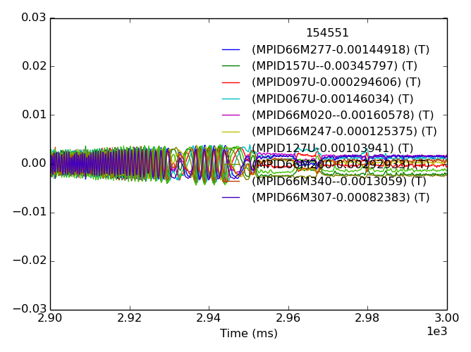
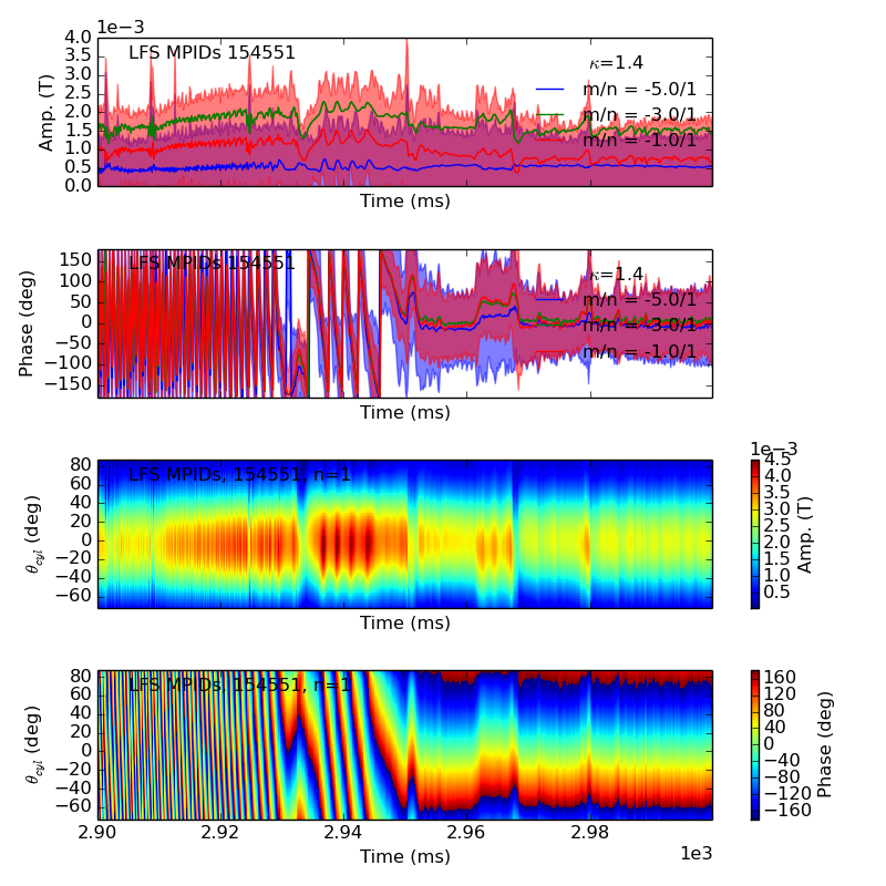
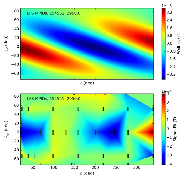
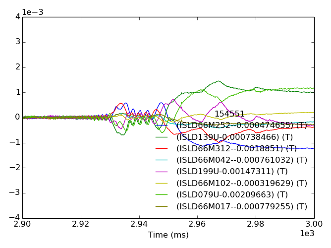
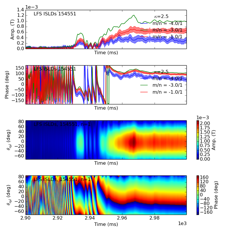


Note that the plots are highly interactive when running this command in an ipython session.
It is highly recomended to check if the result is consistent for various geometries (i.e. basis functions).
>>> emt=quicktorque(154551,base=[2900,2928],xlim=[2900,3000],geom='local',
...                 exclude=['MPID66M307'],ns=[1],ms=[-10,10],display=False)
Calling set_data for sesnors in MPID66M array.
Calling remove_baseline for sesnors in MPID66M array.
Re-forming ModeFit
Condition number = 1.45
Calling set_data for sesnors in MPID67A array.
Calling remove_baseline for sesnors in MPID67A array.
Re-forming ModeFit
Condition number = 1.22
Calling set_data for sesnors in MPID67B array.
Calling remove_baseline for sesnors in MPID67B array.
Re-forming ModeFit
Condition number = 1.22
Calling set_data for sesnors in MPID79A array.
Calling remove_baseline for sesnors in MPID79A array.
Re-forming ModeFit
Condition number = 1.22
Calling set_data for sesnors in MPID79B array.
Calling remove_baseline for sesnors in MPID79B array.
Re-forming ModeFit
Condition number = 1.11
Forming 2D fit from collection of arrays
Calling set_data for sesnors in ISLD66M array.
Calling remove_baseline for sesnors in ISLD66M array.
Re-forming ModeFit
Condition number = 1.08
Calling set_data for sesnors in ISLD67A array.
Calling remove_baseline for sesnors in ISLD67A array.
Re-forming ModeFit
Condition number = 1.11
Calling set_data for sesnors in ISLD67B array.
Calling remove_baseline for sesnors in ISLD67B array.
Re-forming ModeFit
Condition number = 1.1
Calling set_data for sesnors in ISLD79A array.
Calling remove_baseline for sesnors in ISLD79A array.
Re-forming ModeFit
Condition number = 1.22
Calling set_data for sesnors in ISLD79B array.
Calling remove_baseline for sesnors in ISLD79B array.
Re-forming ModeFit
Condition number = 1.11
Forming 2D fit from collection of arrays
Interpolating Amp and Phase to theta
Interpolating Amp and Phase to theta
>>> flocal = emt.plot()
Plotting stress
n = 1
>>> flocal.savefig(__packagedir__+'/doc/examples/stress_local.png')
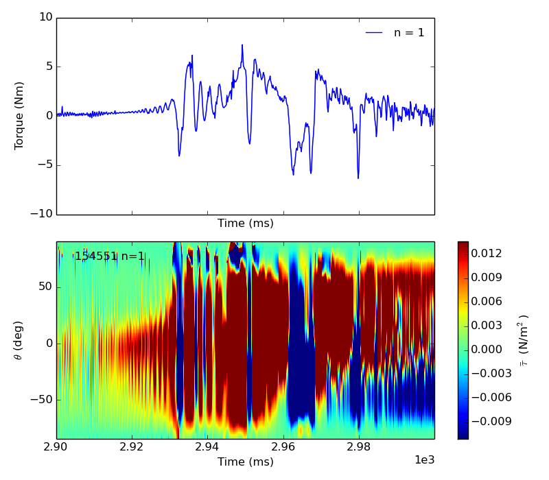
Remember that the spherical harmonics are limited so |m|>n.
>>> emt = quicktorque(154551,base=[2900,2928],xlim=[2900,3000],geom='sphere',
...                   exclude=['MPID66M307'],ns=[1],ms=[-10,-5,-1],display=False)
Calling set_data for sesnors in LFS MPIDs array.
Calling remove_baseline for sesnors in LFS MPIDs array.
Re-forming ModeFit
OPTIMIZED M [-10  -7  -4]
Condition number = 2.98
Calling set_data for sesnors in LFS ISLDs array.
Calling remove_baseline for sesnors in LFS ISLDs array.
Re-forming ModeFit
OPTIMIZED M [-10  -7  -6]
Condition number = 1.83
Interpolating LFS MPIDs fit Amp and Phase to theta
Interpolating LFS ISLDs fit Amp and Phase to theta
>>> fsph = emt.plot()
Plotting stress
n = 1
>>> fsph.savefig(__packagedir__+'/doc/examples/stress_sphere.png')
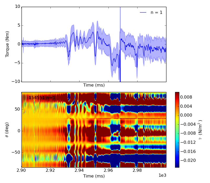
If we showed the fits, we would see the spherical harmonics produce a dubious poloidal field structure. The qualitative agreement between the local and cylindrical harmonics fits is encouraging, despite some qualitative differences.
Bases: object
Class for the computation and visualization of 2D Maxwell Stress fits across the DIII-D vessel.
Note
Maps to ‘greater cylinder’ with r=2.395, which is 3.3cm inside R0 midplane and just inside all points of R+/-1.
Plot time evolution of EM torque.
Additional kwargs passed to matplotlib pcolormesh.
Update both fits, and re-formulate the maxwell stress using the updated fits.
All args and kwargs passed to fit.update
Returns:
- il : bool.
- Calculate torque on lower I-coil array.
Return a modeled torque.
Here “I” is the total effective current I_c+I_ef.
Retrieve magnetics data and calculate toroidal torque from maxwell stress at the vessel wall. All calculations are done using the module’s differenced_arrays (bp/br_differenced_arrays if geom is ‘local’).
The stress is calculated using ‘flat’ geometry at the inner wall.
Choose poloidal variable:
Additional kwargs passed to MaxwellStress initialization.
Tools for fitting response functions to DIII-D magnetics calibration data.
The purpose of this module is simultaneous DC and AC compensation of magnetics data. The module itself provides tools for fitting response functions to DIII-D magnetics calibration data. For further details on the use of response functions please see the presentation Response Function Compensation for DIII-D 3D Magnetics.
A collection of response functions is pickled in this package, and the compensation process is automated in the magnetic Sensor objects. So it is rare that a user would need to interact with this module directly.
Here is example of how to for a response function from a DC calibration shot and apply it to compensate a signal by hand.
>>> d = Data('ISLD66M072',152945,quiet=0)#.remove_baseline(8600,9400,True)
x0(ms) ISLD66M072()
>>> c79 = Data('pcc79',152945,quiet=0)
t(ms) PCC79( )
>>> rlsq,fr = resp_lstsq(d,c79,display=True,smth=0.0)
PCC79-(ISLD66M072-7.33724E-05)
solving least sq matrix eq.
  shape: 13919 = 13919X3976 dot 3976
forming interpolation function
t0 = 1701.34997559 ms,    fmax = 9.94174757282 kHz
R(0) = -1.0222e-06
>>> fr.savefig(__packagedir__+'/doc/examples/response_function_isld66m072-c79_rlsq.png')

>>> c2 = Data('pcc79',153236,quiet=0)
t(ms) PCC79( )
>>> d2 = Data('ISLD66M072',153236,quiet=0)
x0(ms) ISLD66M072()
>>> comp,f = compensate_sensor_coil(d2,c2,rlsq,xlim=(-750,2.5e3),display=True)
Interpolating R
Integrating R(t-tau)*V'(tau)
>>> f.savefig(__packagedir__+'/doc/examples/response_function_isld66m072-c79_compensation.png')

Note that the compensation has a new baseline, which should be removed before any further analysis.
A running to do list:
Compensate a magnetic sensor data object for each of the I-coils.
Additional kwargs passed to each compensate function.
Compensate pickup from 3D coils for magnetics data object.
Calculate a response function.
Limits x axis to 1000 points (fmax set by xrng in this case).
Create a R(t-tau) response function interpolator with tflat ms of active data and a R(0) constant-value fill value for t>300ms.
Note
x axis of interpolator is limited to 1000 pts for speed. This corresponds to accuracy up to ~3kHz.
- Arguments:
- sdat : obj.
- Data object for magnetic sensor
- cdat : obj.
- Data object for coil current (pc-pointnames!)
- Key Word Arguments:
- xlim : list.
- Set range for fit [xstart,xend]
- Default is 200 ms pre-spike in cdat.
- dx : float.
- x axis spacing
- Defaults to min of the data axis spacings or 0.3 to satisfy 1000pt constraint.
- display :bool
- Plot and print information on intermediate steps.
- base : float.
- Baseline span in ms.
- smth : float.
- Smoothing of data in ms.
- tflat : float.
- Time before R is assumed to have flatlined in ms.
- display: bool.
- Print and plot steps along the way.
- details : bool.
- Return tuple containing std,fmax,fmax(psd>0)
Copied from http://www.scipy.org/Cookbook/SignalSmooth
Smooth the data using a window with requested size.
This method is based on the convolution of a scaled window with the signal. The signal is prepared by introducing reflected copies of the signal (with the window size) in both ends so that transient parts are minimized in the begining and end part of the output signal.
- x : ndarray.
- the input signal
Examples:
>>> t=np.linspace(-2,2,50)
>>> x=np.sin(t)+np.random.randn(len(t))*0.1
>>> y=smooth(x)
see also:
numpy.hanning, numpy.hamming, numpy.bartlett, numpy.blackman, numpy.convolve scipy.signal.lfilter
| Authors: | S. Haskey, N. Logan, J. Hanson |
|---|
This module is essentially a pythonification of IDL tranfer function routines administrated by J. Hanson. The module was original developed by S. Haskey, and re-written for the magnetics package by N. Logan.
The purpose of this module is AC compensation. For further details on the use of transfer functions please see the presentation Progress in determining ac coil-sensor couplings for 2012.
To demonstrate compensating a single sensor - coil coupling, we look at a 10Hz vacuum shot from 2013.
>>> probe = 'ISLD67B072'
>>> coil = 'IL90'
>>> probedata = Data(probe,153580,quiet=0)
x0(ms) ISLD67B072()
>>> xlim = (2e3,4e3)
>>> compdata1,f1 = compensate_sensor_coil(probe,probedata,coil,xlim=xlim,display=True,pair=True)
***************IL90-ISLD67B072***************
Time axis from 2e+03 to 4e+03 with stepsize 0.05
WARNING: Using pair compensations
Using data from /u/hansonjm/var/data/transfers/tf2013_pair.h5
Using LISLD079 key from h5 file for sensor ISLD67B072
Warning: Dataset does not have multiple of 16 items - continuing, vers = 1
sp: ['-3.30e+03 0.00e+00i', '-3.37e+02 0.00e+00i']
sz: ['-6.88e+02 0.00e+00i']
sk: ['1.67e-03']
b_s: ['1.67e-03', '1.15e+00']
a_s: ['1.00e+00', '3.64e+03', '1.11e+06']
zpk2tf finished
b_z: ['3.88e-08', '1.31e-09', '-3.75e-08']
a_z: ['1.00e+00', '-1.83e+00', '8.33e-01']
bz and az found
t(ms) IL90( )
RMS for coil: 1.176091e+03, sensor: 1.000147e-03,  transfer: 1.194807e-03
Coil freq = 9.77
>>> f1.savefig(__packagedir__+'/doc/examples/tranfer_function_ISLD67B072-IL90_example.png')
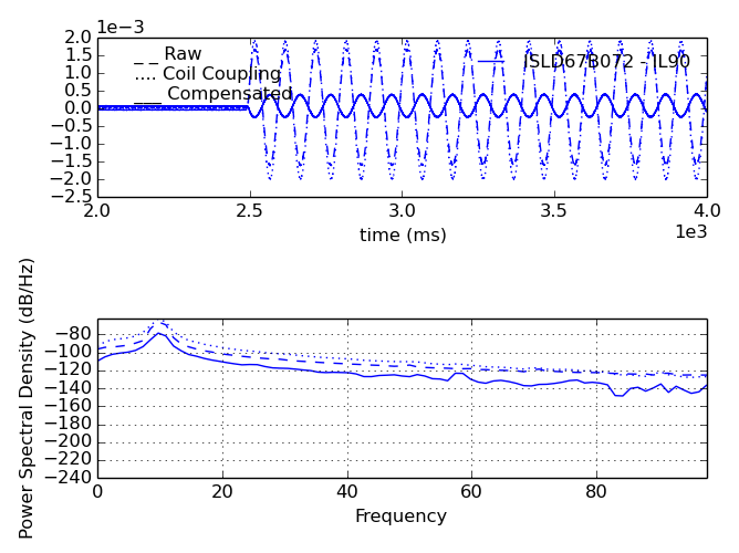
We see here that using the display option generates a good deal of information in the command line, as well as some helpful figures.
In this case, we have already choosen a coupling that clearly dominated the sensor signal. Still, if we wanted to remove all the 3D coil couplings (as we usually do!) we could call the ready-to-use wrapper function,
>>> compdata = compensate(probe,probedata,xlim=xlim,pair=True)
WARNING: Using pair compensations
Using LISLD079 key from h5 file for sensor ISLD67B072
t(ms) IU30( )
t(ms) IU90( )
t(ms) IU150( )
t(ms) IL30( )
t(ms) IL150( )
t(ms) C79( )
t(ms) C139( )
t(ms) C199( )
>>> fall = probedata.plot(label='Raw Signal')
>>> fall = compdata.plot(label='Compensated Signal',figure=fall)
>>> fall.axes[0].set_xlim(*xlim)
(2000.0, 4000.0)
>>> fall.savefig(__packagedir__+'/doc/examples/tranfer_function_ISLD67B072_compensate_example.png')
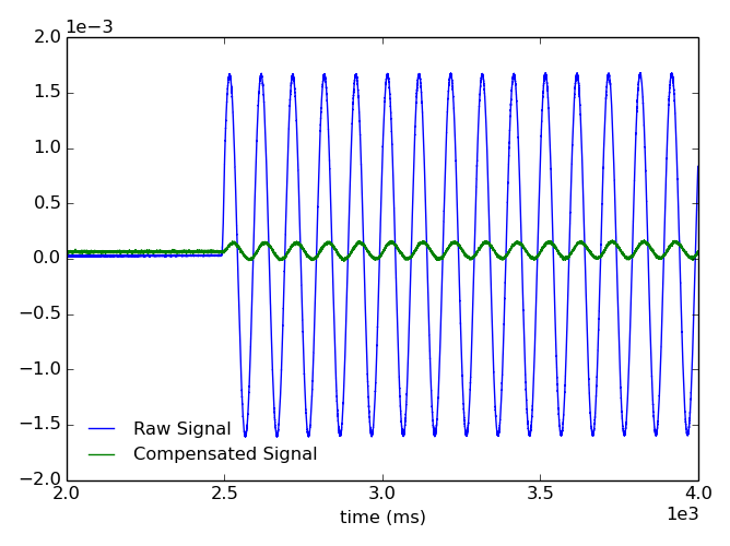
The resulting Data object is fully compensated for IU, IL, and C coil couplings. Note, that the displayed output warns that the only couplings available are even-pair (of the 3D field coils) couplings. That is fine for our case, but be wary of false compensation if applying 3D fields with odd toroidal mode numbers! There are also many warnings about failed searches for coupling data, these are not recorded to (as suggested) to weak coupling.
Return a digital filter from an analog filter using the bilinear transform. The bilinear transform substitutes (z-1) / (z+1) for s.
Compensate a magnetic sensor data object for each of the 3D coils.
Automatically attempts pair compensation if single coil compensation data not available.
Compensate a magnetic sensor data object for a single 3D coil.
Get the couplings between sensor_name and coil_name from a h5 object.
Normalize polynomial representation of a transfer function.
If values of b are too close to 0, they are removed. In that case, a BadCoefficients warning is emitted.
This function has been copied out of scipy with the ‘while’ part below commented out - hopefully this makes some difference to the badly conditioned filter co-eff problem.
b : ndarray.
a : ndarry.
Get the coil signal, interpolate it to time axis, and return the coupling to the sensor using scipy.lfilter(a_z,b_z,coil_current_data).
Get the z-domain transfer function sensor_name and coil_name from a h5 object.
Sinusoidal regression analysis to find the amplitude and phase of the coil frequency in the plasma component of the signal.
Collection of general data collection, manipulation, and visualization tools.
This module builds on the pyD3D data module classes using a copy of the original module stored as ‘data_patched’. This allows additional methods to be introduced into the Data class object through the parent Data_Base within magdata without modification to the data module Data_Base object.
Modifications include addition of a matplotlib based ‘plot’ method (see plot), ‘remove_baseline’ method (see rmbase), and ‘vs’ (see avb).
Bases: data.Data
Modified data.Data class, with support for combination or manipulation directly in the point name.
Modified defaults are: do_search=0,quiet=1.
Additional methodtypes include: vs, remove_baseline and plot.
ORIGINAL DOCUMENTATION:
Data( # CLASS DATA: READ IN AND MANIPULATE GRIDDED DATA STRUCTURES (GENERALLY FROM MDS+ SIGNAL NODES) Data_Init, # CLASS DEFINING FORM OF INSTANCES AND INIT (READS MDS+ DATA) SEE data_init MODULE Data_Base, # CLASS DEFINING BASIS MATH FUNCTION OVERLOADS, SEE data_base MODULE InterpolatingFunction_func, # SUBCLASS OF data_base.InterpolatingFunction USED
# TO CREATE A CALL METHOD WHICH INTERPOLATES THE DATA)
Data.__init__( # # CREATE A Data CLASS INSTANCE # If arguments are given, data in instance is read from MDS+ or PTDATA (D3D only). # If no arguments are given returns an instance with only internal structure to hold data. # Default attributes: # self.xunits = [‘’] : x units, (MDS+ only) # self.xname = [‘’] : x names, == [‘x0’,’x1’,..] # self.x = [] : x values (numpy arrays) # self.xerror = [] : x errors (MDS+ only) = [None, None,..] if None # self.nx = 1 : Number of x values # self.yunits = ‘’ : y units (MDS+ only) # self.yname = ‘’ : y name = pt # self.y = None : y value (numpy array): shape = (len(xn), len(xn-1) ... len(x0)) # self.yerror = None : y error (MDS+ only) = None if None # self.yaux = None : Auxillary y data, e.g. measurement location, shape=[n_attributes]+y.shape # self.yaux_doc=None : Auxillary y data documentation, one string in list for each attribute # self.shot = shot : shot # self.build = ‘’ : String used to rebuild instance for a diff shot with rebuild() # self.islice = ‘’ : Slice islice value. If xslice was used this is the resulting islice. # self.xorder = 0 : Order of x variables in MDS+ relative to structure of y variable # For xorder=0, x0 corresponds to y index with fastest variation in # memory (ala Fortran), xorder=1 is reversed. Used for NSTX data only # self.xext = [] : In cases where some x is more than 1D (e.g. time dependent spacial axis # is used on some EFIT points on NSTX) xext contains the full 2D x data # while self.x contains self.xext[0,:] # self.xerrorext=[] : As for xext but for x error bars # self.xshape = None : For cases where some x are more than 1D contains shape info for x # !!!!!!!! THESE ATTRIBUTES ARE NOLONGER READ AS DIRECT PTDATA READS ARE NOLONGER SUPPORTED !!!!!!!!! # For results read with PTDATA using Ptdata.py (rather than the MDS+ TDI interface) also have # self.t_domains = Timing domains: [ (tmin0,tmax0,dt0), (tmin1,tmax1,dt1), ... ] # self.descript = Description of point stored in ptdata # self.shot_time = Time of shot (string 12:00:00) # self.shot_date = Date of shot (3/31/2005) # Instance can also contain other attributes which exist as subnodes to the data node in MDS+, # a common example of this are subnodes correspoinding to fit parameters in which case a call back # function is created for the instance on initialization. Any number of singnal subnode layers are # allowed and for each signal subnode layer one layer of numeric or text subnodes is allowed. # self, pt = ‘’, # Point Name. Can be either a string, or tuple or list of lenght 2 or 3.
# If a tuple or list the first element must be the MDS+ minpath or # PTDATA pointname and the second element the MDS+ tree (use PTDATA for # the tree for ptdata points). The optinal third element of pt is the # MDS+ minpath to the error bar. # Examples: # x=Data([‘ip’,’ptdata’],98893) : PTDATA point # x=Data([‘ipmhd’,’efit01’],98893): MDS+; ipmhd is a tagname (ipmhd also) # x=Data([‘tsne_core’,’electrons’,’tsne_e_core’],98893): Error bars in sne_e_core # x=Data([‘.p4500_e8099:nedatpsi’,’profdb_ped’],98889): MDS+ full path # If pt is a string must be the MDS+ full path including the tree name, # the MDS+ minpath, or PTDATA pointname. If full path including tree is not # given, tree is looked up or guessed. # Examples: # x=Data(‘ip’,98893)=Data(‘ptdata::topip’,98893) # x=Data(‘ipmhd’,98893)=Data(‘d3d::topipmhd’,98893)=Data(‘d3d::topipmhd’,98893) # x=Data(‘profdb_ped::top.p4500_e8099:nedatpsi’,98889) # Search sequence: # 1) Use dictionary in file ~/MySignals or loaded into variable _MySignals # of the form { name:[path,tree,err_path] } # 2) Look up in postgreSQL tables, # 3) Try using MDSPLUS_BASE_TREE (All trees are subtrees of the mdsplus base tree), # 4) Try using PTDATA (DIII-D only), # 5) Prompt for wildcard search in postgreSQL table (if do_search = 1). # pt can also be entered initially with wildcards to start a search: # * or % matches any length string, ~ matches a single charactershot = None, # Shot Number do_search = 1, # Search data base (1) or error out (0) if point not found quiet = 0, # =1 Don’t print diagnostic info open_tree = 1, # if 0 then don’t open or close MDS+ tree,
# useful if multiple reads from same treesubnodes = 1, # Read subnodes if they exist, if 0 don’t try to get them (faster) error_of = 1, # Read error bars for x and y if they exist, if 0 don’t try to get them (faster) units = 1, # Read units for x and y if they exist, if 0 don’t try (faster) xorder = 0, # Order of x variables in MDS+ relative to structure of y variable
# For xorder=0, x0 corresponds to y index with fastest variation in # memory (ala Fortran), xorder=1 is reversed. Used for NSTX data only
- save_xext = 0, # Save the extended x (and xerror). For some NSTX data radial absissa values
- # are given as functions of time as 2-D arrays. __init__ reduces this to 1-D # x axes (using t index 0) but can save the time dependent x values in xext, xerrorext # if save_xext = 0 then only the shape of these arrays are saved and they are # reconstructed (sort of) on mdsput by expanding the tindex 0 saved in x,xerror
- islice = ‘’, # Slice on index values in MDSplus (not python) form,
- # e.g. ‘[3:7:2,*,20]’ slices x0 from index 3 to 7 inclusive by 2, all if x1, # and index 20 on x2: a 2d array is then returned. note that for slice to work # the abscissa must be ordered the same as the y dimensions: see xorder.
- xslice = ‘’, # Like islice but uses actural axis values. Skips are still done in terms of an
- # index: e.g. xslice=’[1200.3:1400.2:3]’ get data with t>=1200.3ms, t<=1400.3ms # and every third point. Data must have ordered abscissa for xslice to work.
tmin = -1.e5, # Min time(ms), ignored if <= -1.e5. Set automatically by xslice. tmax = 1.e5, # Max time(ms), ignored if >= 1.e5. Set automatically by xslice. # # EXTRAS FOR PTDATA POINTS ONLY. ONLY FOR D3D. SEE Ptdata MODULE DOCUMENTATION use_libd3 = False, # Use libd3 directly rather than through an mdsvalue call. This can be faster
# and does not load the mdsplus server, however more complex data structures in # ptdata are not supported.source = ‘.PLA’, # Data source for ptdata, .PLA is everything (slower search) ical = 1, # Ptdata calibration code: 1=physical units, 2=volts, 0=bits tcode = ‘d’, # Data type to return for ptdata. # # ENVIRONMENTAL VARIABLES CONTROLING INITIALIZATION # MDS_SERVER : IP address of the MDSplus server. # If using local MDS+ trees (or thick client through localhost) use MDS_SERVER=”none” # MDS_BASE_TREE: Base MDS+ tree. If not set defaults to d3d for atlas and cmod for cmod server # MDS_SIGNAL_TABLE: Table on postgreSQL server to search for MDS+ path and tree. # Can also be a series of tables to search separated by path deliminators, e.g. # signame_d3d:signame_cmod. If # rather than : is used to separate the table names search # stops at table where name is first resolved otherwise last matchin value is used. # NO_PGCONNECT: If set suppresses direct connection to the postgreSQL server for point searches. # PGHOST: PostgreSQL server IP address for looking up tree names from point names. # PGPORT: PostgreSQL server connection port. # PGDATABASE: PostgreSQL database looking up tree names from point names. # TOKAMAK: Get data from this experiment. One of (‘D3D’,’NSTX’,’CMOD’,’JET’). This is set # automatically if users IP is in the domain for the experiment (to avoid this # set TOKAMAK=NONE). If TOKAMAK is in (‘D3D’,’NSTX’,’CMOD’,’JET’) then # MDS_SERVER, MDS_BASE_TREE, MDS_SIGNAL_TABLE, PGHOST, PGPORT, PGDATABASE # are all set automatically and do not need to be set as environmental varialbles. # VPN_ACTIVE: When remotely connecting to one of the specific experiments, a Postgresql database # connection is only attemted when VPN_ACTIVE is set. # )
Uses scipy.signal.firwin to design a spectral filter and then applies it to signal. Assumes 1D data. Overrides nyq, using the first time step in data.x[0] to calculate the nyquist frequency. All frequency cutoffs are thus in kHz, and must be between 0 and the nyquist frequency.
Suggested values : numtaps=40
Arguments and Key word arguments are taken from scipy.signal.firwin. Documentation below:
FIR filter design using the window method.
This function computes the coefficients of a finite impulse response filter. The filter will have linear phase; it will be Type I if numtaps is odd and Type II if numtaps is even.
Type II filters always have zero response at the Nyquist rate, so a ValueError exception is raised if firwin is called with numtaps even and having a passband whose right end is at the Nyquist rate.
Set to True to scale the coefficients so that the frequency response is exactly unity at a certain frequency. That frequency is either:
scipy.signal.firwin2
Low-pass from 0 to f:
>> from scipy import signal
>> signal.firwin(numtaps, f)
Use a specific window function:
>> signal.firwin(numtaps, f, window='nuttall')
High-pass (‘stop’ from 0 to f):
>> signal.firwin(numtaps, f, pass_zero=False)
Band-pass:
>> signal.firwin(numtaps, [f1, f2], pass_zero=False)
Band-stop:
>> signal.firwin(numtaps, [f1, f2])
Multi-band (passbands are [0, f1], [f2, f3] and [f4, 1]):
>> signal.firwin(numtaps, [f1, f2, f3, f4])
Multi-band (passbands are [f1, f2] and [f3,f4]):
>> signal.firwin(numtaps, [f1, f2, f3, f4], pass_zero=False)
Returns natural logarithm of data.
..note: By including this, we enable the numpy function to be applied directly to a data object (i.e. np.log(density)).
Plot data.Data class object in using customized matplotlib methods (see pypec.moplot).
Additional kwargs passed to matplotlib.Axes.plot (1D) or matplotlib.Axes.pcolormesh (2D) functions.
..note: Including the ‘marker’ key in kwargs uses matplotlib.Axes.errorbar for 1D plots when data has yerror data.
Plot Power Spectrum Density of data.Data class object using matplotlib methods (see pypec.moplot).
Additional kwargs passed to matplotlib.Axes.psd
Subtracts a uniform base value from the signal data where the base is an avarage of the amplitude over a specified time period.
Create a data object consisting of data a vs. data b.
Examples:
If you want the beam torque as a function of rotation
>>> rotation = Data("-1*'cerqrotct6'/(2*np.pi*1.69)",153268,yunits='kHz',quiet=0)
SUBNODES: ['label', 'multiplier', 'tag4d', 'units', 'variable']
x0(ms) cerqrotct6(km/s)
>>> tinj = -2.4*Data('bmstinj',153268,quiet=0).smooth(100)
t(ms) bmstinj( )
>>> t_v_rot = data_vs_data(tinj,rotation)
>>> t_v_rot.xunits
['kHz']
Uses scipy.signal.firwin to design a spectral filter and then applies it to signal. Assumes 1D data. Overrides nyq, using the first time step in data.x[0] to calculate the nyquist frequency. All frequency cutoffs are thus in kHz, and must be between 0 and the nyquist frequency.
Suggested values : numtaps=40
Arguments and Key word arguments are taken from scipy.signal.firwin. Documentation below:
FIR filter design using the window method.
This function computes the coefficients of a finite impulse response filter. The filter will have linear phase; it will be Type I if numtaps is odd and Type II if numtaps is even.
Type II filters always have zero response at the Nyquist rate, so a ValueError exception is raised if firwin is called with numtaps even and having a passband whose right end is at the Nyquist rate.
Set to True to scale the coefficients so that the frequency response is exactly unity at a certain frequency. That frequency is either:
scipy.signal.firwin2
Low-pass from 0 to f:
>> from scipy import signal
>> signal.firwin(numtaps, f)
Use a specific window function:
>> signal.firwin(numtaps, f, window='nuttall')
High-pass (‘stop’ from 0 to f):
>> signal.firwin(numtaps, f, pass_zero=False)
Band-pass:
>> signal.firwin(numtaps, [f1, f2], pass_zero=False)
Band-stop:
>> signal.firwin(numtaps, [f1, f2])
Multi-band (passbands are [0, f1], [f2, f3] and [f4, 1]):
>> signal.firwin(numtaps, [f1, f2, f3, f4])
Multi-band (passbands are [f1, f2] and [f3,f4]):
>> signal.firwin(numtaps, [f1, f2, f3, f4], pass_zero=False)
Returns natural logarithm of data.
..note: By including this, we enable the numpy function to be applied directly to a data object (i.e. np.log(density)).
Common shot-overvieiew signals.
dict. Contains data.Data type objects for
Plot data.Data class object in using customized matplotlib methods (see pypec.moplot).
Additional kwargs passed to matplotlib.Axes.plot (1D) or matplotlib.Axes.pcolormesh (2D) functions.
..note: Including the ‘marker’ key in kwargs uses matplotlib.Axes.errorbar for 1D plots when data has yerror data.
Plot the 3D field coil currents for a shot.
Plot Power Spectrum Density of data.Data class object using matplotlib methods (see pypec.moplot).
Additional kwargs passed to matplotlib.Axes.psd
Subtracts a uniform base value from the signal data where the base is an avarage of the amplitude over a specified time period.
Provides visualization tools for hardcoded geometric features of the DIII-D tokamak.
Used in the magnetics package to provide context for magnetic probe locations.
To visualize a surface object,
>>> f = vessel.plot3d(wireframe=True, linewidth=0.1)
>>> f.savefig(__packagedir__+'/doc/examples/d3dgeometry_vessel_example.png')
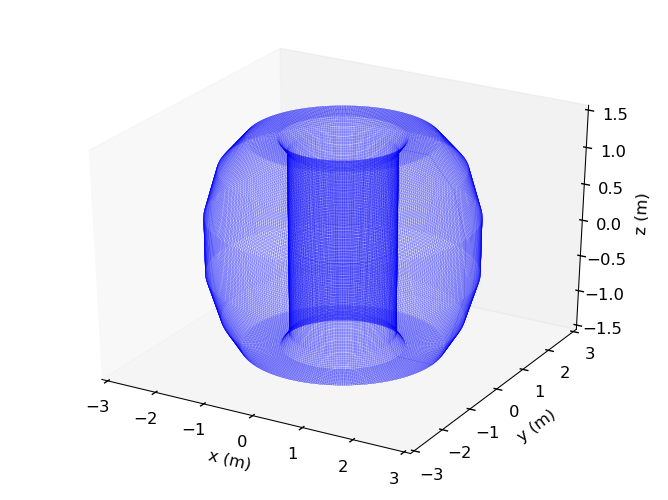
An geometric class with standardized visualization methods for an axi-symmetric surface defined by attributes r and z.
Displays the poloidal cross section of the surface as a line on r,z plot.
Valid kwargs are matplotlib.pyplot plot keyword arguments.
Plots the surface in as a mesh 3 dimensional space.
- Key Word Arguments:
- wireframe : bool
- Use matplotlib Axes3D.plot_wireframe instead of plot_surface.
Valid kwargs are Axes3D.plot_wireframe or Axes3D.plot_surface keywords.
Collection of modified matplotlib functions and objects.
Highlights include:
- New “printlines” Figure method for saving displayed data to ascii tables.
- Complex argument handling in Axes “plot” method.
- Speed increases with dynamic downsampling of large data in interactive Axes objects.
- Customized defualts using use_gridspec=True, for consistency with autolayout
Note
Although almost entirely self-contained, this module does modify the matplotlib.lines.Line2D object by adding a downsample method.
Plot complex arguments.
>>> f,ax = subplots()
>>> lines = ax.plot(np.arange(10)*(1+0.5j),label='complex_arg')
>>> f.savefig(__packagedir__+'/doc/examples/magplotlib_complexargs.png')
Automatically resize plot axes to fit labels in figure.
>>> xlbl = ax.set_xlabel('X AXIS')
Plot huge data sets quickly.
>>> x = np.linspace(0,9,1e5)
>>> data = np.arange(1e5)/1.5e4+(np.random.rand(1e5)-0.5)
>>> newline = ax.plot(x,data,label='large data set')
>>> f.savefig(__packagedir__+'/doc/examples/magplotlib_complexargs2.png')
This plots a line capped at 1000-pts by default. The maximum number of points is maintained as you manipulate the axis, so zooming in will provide you with new points and increased detail until the window samples fewer than that many points in the orginal data. The first two lines, for instance, contain only their original 10 points (not 1000 interpolated points).
Modified pyplot colorbar for default use_gridspec=True.
ORIGINAL DOCUMENTATION
Add a colorbar to a plot.
Function signatures for the pyplot interface; all but the first are also method signatures for the colorbar() method:
colorbar(**kwargs)
colorbar(mappable, **kwargs)
colorbar(mappable, cax=cax, **kwargs)
colorbar(mappable, ax=ax, **kwargs)
arguments:
- mappable
- the Image, ContourSet, etc. to which the colorbar applies; this argument is mandatory for the colorbar() method but optional for the colorbar() function, which sets the default to the current image.
keyword arguments:
- cax
- None | axes object into which the colorbar will be drawn
- ax
- None | parent axes object(s) from which space for a new colorbar axes will be stolen. If a list of axes is given they will all be resized to make room for the colorbar axes.
- use_gridspec
- False | If cax is None, a new cax is created as an instance of Axes. If ax is an instance of Subplot and use_gridspec is True, cax is created as an instance of Subplot using the grid_spec module.
Additional keyword arguments are of two kinds:
axes properties:
Property Description orientation vertical or horizontal fraction 0.15; fraction of original axes to use for colorbar pad 0.05 if vertical, 0.15 if horizontal; fraction of original axes between colorbar and new image axes shrink 1.0; fraction by which to shrink the colorbar aspect 20; ratio of long to short dimensions anchor (0.0, 0.5) if vertical; (0.5, 1.0) if horizontal; the anchor point of the colorbar axes panchor (1.0, 0.5) if vertical; (0.5, 0.0) if horizontal; the anchor point of the colorbar parent axes. If False, the parent axes’ anchor will be unchanged colorbar properties:
Property Description extend [ ‘neither’ | ‘both’ | ‘min’ | ‘max’ ] If not ‘neither’, make pointed end(s) for out-of- range values. These are set for a given colormap using the colormap set_under and set_over methods. extendfrac [ None | ‘auto’ | length | lengths ] If set to None, both the minimum and maximum triangular colorbar extensions with have a length of 5% of the interior colorbar length (this is the default setting). If set to ‘auto’, makes the triangular colorbar extensions the same lengths as the interior boxes (when spacing is set to ‘uniform’) or the same lengths as the respective adjacent interior boxes (when spacing is set to ‘proportional’). If a scalar, indicates the length of both the minimum and maximum triangular colorbar extensions as a fraction of the interior colorbar length. A two-element sequence of fractions may also be given, indicating the lengths of the minimum and maximum colorbar extensions respectively as a fraction of the interior colorbar length. extendrect [ False | True ] If False the minimum and maximum colorbar extensions will be triangular (the default). If True the extensions will be rectangular. spacing [ ‘uniform’ | ‘proportional’ ] Uniform spacing gives each discrete color the same space; proportional makes the space proportional to the data interval. ticks [ None | list of ticks | Locator object ] If None, ticks are determined automatically from the input. format [ None | format string | Formatter object ] If None, the ScalarFormatter is used. If a format string is given, e.g., ‘%.3f’, that is used. An alternative Formatter object may be given instead. drawedges [ False | True ] If true, draw lines at color boundaries. The following will probably be useful only in the context of indexed colors (that is, when the mappable has norm=NoNorm()), or other unusual circumstances.
Property Description boundaries None or a sequence values None or a sequence which must be of length 1 less than the sequence of boundaries. For each region delimited by adjacent entries in boundaries, the color mapped to the corresponding value in values will be used.
If mappable is a ContourSet, its extend kwarg is included automatically.
Note that the shrink kwarg provides a simple way to keep a vertical colorbar, for example, from being taller than the axes of the mappable to which the colorbar is attached; but it is a manual method requiring some trial and error. If the colorbar is too tall (or a horizontal colorbar is too wide) use a smaller value of shrink.
For more precise control, you can manually specify the positions of the axes objects in which the mappable and the colorbar are drawn. In this case, do not use any of the axes properties kwargs.
It is known that some vector graphics viewer (svg and pdf) renders white gaps between segments of the colorbar. This is due to bugs in the viewers not matplotlib. As a workaround the colorbar can be rendered with overlapping segments:
cbar = colorbar()
cbar.solids.set_edgecolor("face")
draw()
However this has negative consequences in other circumstances. Particularly with semi transparent images (alpha < 1) and colorbar extensions and is not enabled by default see (issue #1188).
Function to connect key_press_event events from matplotlib to custom functions.
Matplotlib defaults (may be changed in matplotlibrc):
keymap.fullscreen : f # toggling keymap.home : h, r, home # home or reset mnemonic keymap.back : left, c, backspace # forward / backward keys to enable keymap.forward : right, v # left handed quick navigation keymap.pan : p # pan mnemonic keymap.zoom : o # zoom mnemonic keymap.save : s # saving current figure keymap.quit : ctrl+w # close the current figure keymap.grid : g # switching on/off a grid in current axes keymap.yscale : l # toggle scaling of y-axes (‘log’/’linear’) keymap.xscale : L, k # toggle scaling of x-axes (‘log’/’linear’) keymap.all_axes : a # enable all axes
My custom function mapping:
popaxes : n #Creates new figure with current axes tighten : t #Call tight_layout bound method for figure
Re-create a given axis in a new figure. This allows, for instance, a subplot to be moved to its own figure where it can be manipulated and/or saved independent of the original.
Print all data in line plot(s) to text file.The x values will be taken from the line with the greatest number of points in the (first) axis, and other lines are interpolated if their x values do not match. Column lables are the line labels and xlabel.
Matplotlib subplots with default sharex=True.
- Additional Key Word Arguments:
- powlim : tuple.
- Axis labels use scientific notion above 10^power.
- useOffset : bool.
- Axis labels use offset if range<<average.
Accepts standargs args and kwargs for pyplot.subplots.
ORIGINAL DOCUMENTATION
Create a figure with a set of subplots already made.
This utility wrapper makes it convenient to create common layouts of subplots, including the enclosing figure object, in a single call.
Keyword arguments:
- nrows : int
- Number of rows of the subplot grid. Defaults to 1.
- ncols : int
- Number of columns of the subplot grid. Defaults to 1.
- sharex : string or bool
- If True, the X axis will be shared amongst all subplots. If True and you have multiple rows, the x tick labels on all but the last row of plots will have visible set to False If a string must be one of “row”, “col”, “all”, or “none”. “all” has the same effect as True, “none” has the same effect as False. If “row”, each subplot row will share a X axis. If “col”, each subplot column will share a X axis and the x tick labels on all but the last row will have visible set to False.
- sharey : string or bool
- If True, the Y axis will be shared amongst all subplots. If True and you have multiple columns, the y tick labels on all but the first column of plots will have visible set to False If a string must be one of “row”, “col”, “all”, or “none”. “all” has the same effect as True, “none” has the same effect as False. If “row”, each subplot row will share a Y axis and the y tick labels on all but the first column will have visible set to False. If “col”, each subplot column will share a Y axis.
- squeeze : bool
If True, extra dimensions are squeezed out from the returned axis object:
- if only one subplot is constructed (nrows=ncols=1), the resulting single Axis object is returned as a scalar.
- for Nx1 or 1xN subplots, the returned object is a 1-d numpy object array of Axis objects are returned as numpy 1-d arrays.
- for NxM subplots with N>1 and M>1 are returned as a 2d array.
If False, no squeezing at all is done: the returned axis object is always a 2-d array containing Axis instances, even if it ends up being 1x1.
- subplot_kw : dict
- Dict with keywords passed to the add_subplot() call used to create each subplots.
- gridspec_kw : dict
- Dict with keywords passed to the GridSpec constructor used to create the grid the subplots are placed on.
- fig_kw : dict
- Dict with keywords passed to the figure() call. Note that all keywords not recognized above will be automatically included here.
Returns:
fig, ax : tuple
- fig is the matplotlib.figure.Figure object
- ax can be either a single axis object or an array of axis objects if more than one subplot was created. The dimensions of the resulting array can be controlled with the squeeze keyword, see above.
Examples:
x = np.linspace(0, 2*np.pi, 400)
y = np.sin(x**2)

# Just a figure and one subplot
f, ax = plt.subplots()
ax.plot(x, y)
ax.set_title('Simple plot')

# Two subplots, unpack the output array immediately
f, (ax1, ax2) = plt.subplots(1, 2, sharey=True)
ax1.plot(x, y)
ax1.set_title('Sharing Y axis')
ax2.scatter(x, y)

# Four polar axes
plt.subplots(2, 2, subplot_kw=dict(polar=True))

# Share a X axis with each column of subplots
plt.subplots(2, 2, sharex='col')

# Share a Y axis with each row of subplots
plt.subplots(2, 2, sharey='row')

# Share a X and Y axis with all subplots
plt.subplots(2, 2, sharex='all', sharey='all')
# same as
plt.subplots(2, 2, sharex=True, sharey=True)