Flux Surfaces and Magnetic Islands
From QED
Many plasma configurations are strongly anisotropic because of the presence of a preferentially-directed magnetic field. If the system has a direction of symmetry, such as toroidal symmetry in tokamaks, then analysis of the system can be greatly simplified by the introduction of a magnetic flux function  . The flux function is chosen such that the magnetic field
  lies on surfaces of constant , called flux surfaces. This is mathematically stated by the condition that

In the plane perpendicular to the direction of symmetry in the system, the magnetic fieldlines are simply contours of constant .
Contents |
General Flux Function Form of the Magnetic Field
Examine the system in a generalized curvilinear coordinate system defined by the coordinates  . The differential displacement vector in such a coordinate system is given by
where the geometric factors  are related to the Cartesian coordinates
  by
by
Working in these generalized coordinates, if  is taken to be the direction of symmetry, then the magnetic field can be written in the form
where  and
and  . This form of trivially satisfies
  , and the factor of
  ensures that
  .
.
In Cartesian coordinates with  -directed symmetry,
  , giving

In cylindrical  coordinates with
  -directed symmetry,
  , so
, so
The ordering is chosen so that the coordinate system is still right handed when  .
.
Relation Between the Flux Function and the Magnetic Vector Potential
The flux function can be related to the magnetic vector potential  , which is given by
Expanding the curl operator in the aforementioned generalized curvilinear coordinates, the above equation becomes
![\nabla\times\mathbf{A} = \frac{1}{h_2 h_3}\left[\frac{\partial(h_3 A_3)}{\partial x_2} - \frac{\partial(h_2 A_2)}{\partial x_3}\right] \mathbf{\hat{e}}_1
+ \frac{1}{h_1 h_3}\left[\frac{\partial(h_1 A_1)}{\partial x_3} - \frac{\partial(h_3 A_3)}{\partial x_1}\right]\mathbf{\hat{e}}_2 + B_3 \mathbf{\hat{e}}_3.](../../images/math/e/9/4/e941b8d88dedce81f67c7dd7352936b9.png)
Because symmetry is assumed along and thus  , the expression for
  becomes

+ B_3 \mathbf{\hat{e}}_3.](../../images/math/0/2/d/02d8bdeb890b33184d8deca85dd158df.png)
Now expand the flux-function form of in a similar manner. Begin with
![\nabla\psi\times\mathbf{\hat{e}}_3 = \left[\frac{1}{h_1}\left(\frac{\partial \psi}{\partial x_1}\right) \mathbf{\hat{e}}_1
+ \frac{1}{h_2}\left(\frac{\partial \psi}{\partial x_2}\right) \mathbf{\hat{e}}_2\right]\times\mathbf{\hat{e}}_3
= \left[\frac{1}{h_2}\frac{\partial}{\partial x_2}\mathbf{\hat{e}}_1 - \frac{1}{h_1}\frac{\partial}{\partial x_1}\mathbf{\hat{e}}_2\right] \psi.](../../images/math/f/5/b/f5b065a478e4e0bdf70c8cc35916b8a3.png)
Substituting the above expression into the flux-function form of gives
![\mathbf{B} = \frac{1}{h_3}\nabla\psi\times\mathbf{\hat{e}}_3 + B_3 \mathbf{\hat{e}}_3 =
\frac{1}{h_3}\left[\frac{1}{h_2}\frac{\partial}{\partial x_2}\mathbf{\hat{e}}_1 - \frac{1}{h_1}\frac{\partial}{\partial x_1}\mathbf{\hat{e}}_2\right] \psi
+ B_3 \mathbf{\hat{e}}_3.
:](../../images/math/5/4/f/54ff6e47341042204c17f1e23522e602.png)
Subtracting the flux-function form of from the vector potential form leaves
![\frac{1}{h_3}\left[\frac{1}{h_2}\frac{\partial}{\partial x_2}\mathbf{\hat{e}}_1 - \frac{1}{h_1}\frac{\partial}{\partial x_1}\mathbf{\hat{e}}_2\right] (h_3 A_3 - \psi) = 0.](../../images/math/d/d/8/dd8a414cab98d1bdcbfeb436f1b603f7.png)
From the above equation, it is clear that, to within a constant,

Consequently, in Cartesian coordinates,  , and in cylindrical coordinates,
  .
.
Time Evolution of the Flux Function in Resistive MHD
Assuming that, as in MHD, the scalar electrostatic potential is negligible due to quasineutrality, Faraday's Law gives the electric field to be

Substituting for  using the generalized Ohm's Law from resistive MHD (
 ) gives
From above,  , so to find
  , examine the component of the above equation:
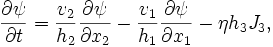
![\frac{\partial \psi}{\partial t} = h_3\frac{\partial A_3}{\partial t} = h_3\bigg[(\mathbf{v}\times\mathbf{B})_3 - \eta J_3\bigg]
= h_3\bigg[ v_2 B_1 - v_1 B_2 - \eta J_3\bigg] = h_3\left[\frac{v_2}{h_2 h_3}\frac{\partial\psi}{\partial x_2} - \frac{v_1}{h_1 h_3}\frac{\partial\psi}{\partial x_1} - \eta J_3\right],](../../images/math/a/0/5/a05e7d9e3907ca77109f61a6b86de52d.png)
where the flux function form of has been used. The final form for is then
Topological Properties of the Flux Function: X-Points, O-Points, and Magnetic Islands
The flux function  can exhibit many of the topological characteristics associated with multi-dimensional functions such as maxima, minima, and saddle points. Maxima and minima in the flux function are called O-points, and saddle points are called X-points. Magnetic fieldlines are contours of constant in the
  plane, so the X- and O-point designations arise because a fieldline forms an "X" shape when passing through and X-point and an "O"-shaped ring when circling an O-point.
The mathematical condition for the existence of an X- or O-point is that

To distinguish between extrema (minima or maxima) and saddle points, use the multi-dimensional second derivative test. Construct the quantity  , which has the form
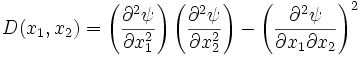
Not sure if this form of is valid for any arbitrary curvilinear coordinate system. The factors could play a non-negligible role in above the expression. Regardless, examining at the point  distinguishes X- and O-points:
- If
 , then is an extremum (an O-point)
- If
 , then is a saddle point (an X-point)
Using this method, all of the X- and O-points in the system can be identified.
X- and O-points in a plasma configuration are accompanied by features known as magnetic islands. These islands are regions of flux that are isolated from the rest of the configuration by a magnetic separatrix. An X-point is the location of closure for this separatrix, so the value of the flux function everywhere on the separatrix is equal to the value of the flux function at the X-point  . An O-point will exist in the interior of the island.
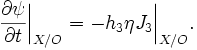
Because  at X- and O-points, the magnetic field will be directed only along the direction of symmetry at these points and the time evolution equation for reduces to simply
Examples
- Generals 2006, Part I, Problem 1
References
- ↑ Kusse, Bruce and Erik Westwig, Mathematical Physics, Wiley (1998). ISBN 0-471-15431-8


