Warning: jsMath requires JavaScript to process the mathematics on this page.
If your browser supports JavaScript, be sure it is enabled.

Perturbation Theory (Quantum Mechanics)

From QED

< PlasmaWiki(Link to this page as [[PlasmaWiki/Perturbation Theory (Quantum Mechanics)]])

Jump to: navigation, search

Only a tiny fraction of problems in quantum mechanics can be be solved analytically. When an exact solution cannot be obtained, one may seek approximate answers through a variety of means, perturbation theory being one of them.

Loosely, it happens that the behavior of most quantum systems changes in a fairly regular way upon a slight modification. When a system can be described by a core part, which is to be solved exactly, or nearly so (perhaps using variational principles to determine the ground-state wavefunction), and a smaller part, called the perturbation, we can apply the methods of perturbation theory to determine in an approximate way the behavior of the perturbed system.

Perturbation Theory also describes a more general mathematical framework for obtaining perturbative solutions to other types of systems.

The core of perturbation theory, as applied to quantum mechanics, is present in the comparatively simple time-independent nondegenerate case. We need to be quite careful around degeneracies -- fortunately we provide a framework which largely handles this for us. There is a cost: we are now required to solve the Eigenvalue Problem directly.

Time-dependent perturbation theory is even more involved, but it allows us to deal with an extraordinary variety of interesting systems (indeed, five nobel prizes have been awarded for resonance of two state systems in time dependent potentials! (I.I.Rabi on Molecular Beams and Nuclear Magnetic Resonance, Bloch and Purcell on B fields in atomic nuclei and nuclear magnetic moments; Townes, Basov, and Prochorov on masers, lasers, and quantum optics; Kastler on optical pumping; and Lauterbur and Mansfield (Medicine) for MRI). One of the most useful formulas to arise out of this topic is Fermi's Golden Rule for transition probabilities.

In what follows we largely follow Sakurai, so please refer to Modern Quantum Mechanics if you're looking for a text.

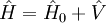
Consider a system describe by a Hamiltonian $\hat{H}$ which may be split like so:

$\hat{H} = \hat{H}_0 + \hat{V}$

The $|n^{(0)}\rang$ . Here we omit this cumbersome notation. Where an expression is ambiguous assume dimensional consistency)</i>

We wish to solve, approximately, the eigenstate problem for the full Hamiltonian.

$(\hat{H}_0 + \lambda \hat{V}) |n\rang = E_n|n\rang$

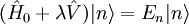
We make use of a parameter $λ$ , which may be 'dialed' from 0 to 1. In practically all systems there is a smooth transition between the perturbed and unperturbed system. (note: for this method to be valid, this eigenitems must be analytic in a complex plane around $λ = 0$ )

As the parameter $λ$ increases from 0, the energy of the nth level shifts from it's unperturbed value. We define the energy shift as

$\Delta_n = E_n - E_n^0$

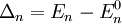
Where we note that $Δ n, E n$ are functions of the perturbation parameter $λ$ . We rearrange the Schrödinger equation like so:

$(E_n^0 - \hat{H}_0)|n\rang = (\lambda \hat{V} - \Delta_n)|n\rang$

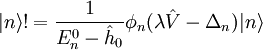
We may invert the operator $\lang n^0|$ )

$\lang n^0|(E_n^0 - \hat{H}_0)|n\rang = E_n^0 - E_n^0 = 0 = \lang n^0|(\lambda \hat{V} - \Delta_n)|n\rang$

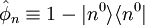
We can define a complementary projection operator $\hat{\phi}_n$ , to project states away from the unperturbed states.

$\hat{\phi}_n \equiv 1 - | n^0 \rang \lang n^0 |$

The operator $\hat{\phi}_n$ to the right.

The following equation is then correct in every dimension except for that in the direction of $| n^0 \rang$

$|n\rang != \frac{1}{E_n^0 - \hat{h}_0} \phi_n(\lambda \hat{V} - \Delta_n) | n \rang$

We correct this by adding a term in the direction of $| n^0 \rang$ .

$|n\rang = c_n(\lambda) | n^0 + \rang \frac{1}{E_n^0 - \hat{h}_0} \hat{\phi}_n(\lambda \hat{V} - \Delta_n) | n \rang$

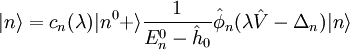
To reduce to the unperturbed equation when $c_n = \lang n^0|n\rang$ . In fact, since the equation is homogeneous $c n$ is a free variable, and we may set $c n (λ) = 1$ and normalize the ket at the end of the calculation.

Simplifying, we obtain the two equations which the rest of the method is based on:

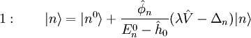
$1: \quad\quad |n\rang = | n^0 \rang + \frac{\hat{\phi}_n}{E_n^0 - \hat{h}_0}(\lambda \hat{V} - \Delta_n) | n \rang$

and from 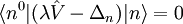$\lang n^0|(\lambda \hat{V} - \Delta_n)|n\rang = 0$ ,

$2: \quad\quad \Delta_n = \lambda \lang n^0|\hat{V}|n\rang\quad{(2)}$

The basic strategy is to expand $|n\rang$ and $Δ n$ in the powers of $λ$ and then match the appropriate coefficients. This is a perfectly valid strategy, since the whole derivation has made no regard to the value of $λ$ , and An Nth Degree Polynomial has N Roots. Thus

$| n \rang = |n^0\rang + \lambda | n^1 \rang + \lambda^2 | n^2 \rang + \dots$

$\Delta_n = \lambda \Delta_n^1 + \lambda^2 \Delta_n^2 + \dots$

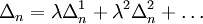
where $| n^m \rang, \Delta_n^m$ stand for the mth order corrections. Substituting our expanded eigenstates and energy shifts into equation 2, and equating the coefficients of powers of $λ$ yields

$O(\lambda^m): \Delta_n^m = \lang n^0|\hat{V}|n^{m-1}\rang$

Turning our attention to an expanded equation 1, we have

$|n^0\rang + \lambda | n^1 \rang + \lambda^2 | n^2 \rang + \dots = |n^0\rang + \frac{\hat{\phi}_n}{E_n^0 - \hat{h}_0}(\lambda \hat{V} - \lambda \Delta_n^1 - \lambda^2 \Delta_n^2 - \dots) \times (|n^0\rang + \lambda | n^1 \rang + \lambda^2 | n^2 \rang + \dots )$

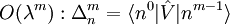
At this point the strategy becomes clear. $\Delta_n^m$ may be evaluated with only the $m - 1$ th order eigenket. The mth order eigenket may be obtained knowing only up to the mth order energy shift. This procedure may continue for as long as is desired (in fact, it may even be possible to evaluate the sum analytically).

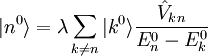
If we write down, to second order, the explicit expansion for $Δ n$ and $|n\rang$ , we can make several interesting qualitative observations.

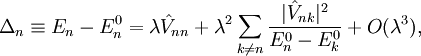
$\Delta_n \equiv E_n - E_n^0 = \lambda \hat{V}_{nn} + \lambda^2 \sum_{k \neq n} \frac{|\hat{V}_{nk}|^2}{E_n^0 - E_k^0} + O(\lambda^3),$

where

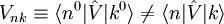
$V_{nk} \equiv \lang n^0|\hat{V}|k^0\rang \neq \lang n | \hat{V} | k \rang$

The matrix elements $V n k$ are taken with respect to the unperturbed kets. For the pertrubed ket, the expansion is

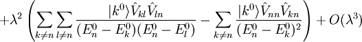
$|n^0\rang = \lambda \sum_{k \neq n} |k^0\rang \frac{\hat{V}_{kn}}{E_n^0 - E_k^0}$

$\quad \quad + \lambda^2 \left({\sum_{k \neq n}\sum_{l \neq n} \frac{|k^0\rang \hat{V}_{kl}\hat{V}_{ln}}{(E_n^0 - E_k^0)(E_n^0 - E_l^0)} - \sum_{k \neq n} \frac{|k^0\rang \hat{V}_{nn}\hat{V}_{kn}}{(E_n^0 - E_k^0)^2}}\right) + O(\lambda^3)$

Examining the last equation closely, we see that the perturbation has the effect of mixing the previously unperturbed eigenkets.

The second order energy shift (the second term in the second last equation) exhibits interesting behavior. The energy levels of kets which are "mixed" by $\hat{V}$ (where $V n k$ is positive) are repelled away from each other. This is a special case of the No-level Crossing Theorem, which states that a pair of energy levels connected by perturbation do not cross as the strength of the perturbation is varied.