QM J04 2
From QED
Two observers in different inertial frames will need
different wave functions to describe the same physical
system. To make things simple we will consider how it
works in one dimension: The first observer uses
coordinates (x,t) and a wave function ψ(x,t) while the second
uses  , v a constant velocity.
The wave functions for the two observers are said to be
related as follows:
, v a constant velocity.
The wave functions for the two observers are said to be
related as follows:
![\hat{\psi}(x^{\prime},t)=\psi(x,t)\exp\left(-\frac{i}{\hbar}\left[mvx-\frac{m}{2}v^{2}t\right]\right)](../../../images/math/5/8/e/58e7a80ed077f3d0511742b6b7065811.png)
Despite its innocuous look (it's just a phase!) this transformation has interesting effects!
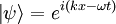
a. Let's verify that it makes sense. Suppose \psi(x,t) is the
wave function for a free particle of momentum p. Show
that  is the wave function of a free particle with a
different momentum. What is its momentum?
is the wave function of a free particle with a
different momentum. What is its momentum?
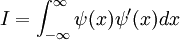
b. Now let's put this to work. Suppose we have a harmonic oscillator in its ground state for t<0 ; its wave function is
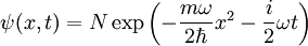
where N is a normalization constant. Suppose that at t=0 the potential suddenly starts to move at velocity v. Because the wave function does not change immediately, it is no longer the ground state wave function of the moving harmonic oscillator. What is the probability of finding the system in the moving ground state at a later time t>0?
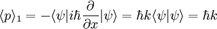
The momentum of the free particle is:
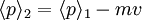
We can find the momentum in the first observer's frame easily:
In the second observer's frame:
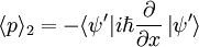
We start just taking:
![\frac{\partial}{\partial x}|\psi^{\prime}\rangle=\frac{\partial}{\partial x}\left(e^{i(kx-\omega t)}\exp\left(-\frac{i}{\hbar}\left[mvx-\frac{m}{2}v^{2}t\right]\right)\right)=\left(ik-imv/\hbar\right)\left|\psi^{\prime}\right\rangle](../../../images/math/8/7/a/87aa9b1cef9ceb84bc184bf460bab14b.png)
Giving:

So:
We can take the new ground state and integrate against the previous ground state, using the sudden approximation to find the probability it is still in the ground state:

![I=\int_{-\infty}^{\infty}N^{2}\exp\left(-\frac{2m\omega}{2\hbar}x^{2}-\frac{2i}{2}\omega t\right)\exp\left(-\frac{i}{\hbar}\left[mvx-\frac{m}{2}v^{2}t\right]\right)dx](../../../images/math/6/e/4/6e4148097e8772ab9d5a8f3c7ccf3ae8.png)
Combining the exponentials and using t=0:
![I=\int_{-\infty}^{\infty}N^{2}\exp\left(-\frac{m}{\hbar}\left[\omega x^{2}+ivx\right]\right)dx](../../../images/math/0/a/8/0a868008d54d08d4b28a92148b7696ae.png)
Completing the square:
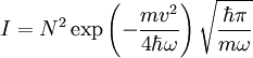
![I=N^{2}\exp\left(-\frac{mv^{2}}{4\hbar\omega} \right)\int_{-\infty}^{\infty}\exp\left(-\frac{m}{\hbar}\left[\omega x^{2}+ivx-\frac{v^{2}}{4\omega}\right]\right)dx](../../../images/math/2/7/b/27b304344d98e52ed2c9a28288cc084a.png)
![I=N^{2}\exp\left(-\frac{mv^{2}}{4\hbar\omega} \right)\int_{-\infty}^{\infty}\exp\left(-\frac{m}{\hbar\omega}\left[\omega x+\frac{iv}{2}\right]^{2}\right)dx](../../../images/math/6/6/7/6674f4ade7a2b73bf5fd7bb88033e9f0.png)
We can now transform to 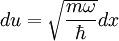 :
:
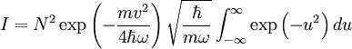
The last integral is just  :
:
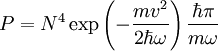
So that the probability is:
This page was recovered in October 2009 from the Plasmagicians page on Prelim_J04_QM2 dated 19:28, 10 April 2007.


