WavesBestiary
From QED
The Waves Bestiary
Sit in reverie, and watch the changing color of the waves that break upon the idle seashore of the mind
- Henry Wadsworth Longfellow
This page is intended to be a summary of the various types of waves encountered in plasma physics. It was originally created by Abe Fetterman, then redone and expanded by Craig Jacobson, and finally moved from LaTeX to the PlasmaWiki. Surely there are errors in this document. Please correct them as they are found. There also seem to be some errors with wiki formatting. Please correct those as well. All the equations are in cgs units because the source material for this is Waves in Plasmas by Stix.
Contents |
Cold Plasma Waves (By ascending frequency)
Alfvén Hydromagnetic Waves
Here we assume  . There are two. One is the \emph{slow}
or \emph{shear} or \emph{torsional} Alfvén wave:
. There are two. One is the \emph{slow}
or \emph{shear} or \emph{torsional} Alfvén wave:

And the other is the \emph{fast} or \emph{compressional} Alfvén wave:

Ion Cyclotron Waves
The slow Alfvén wave is cutoff, and the dispersion relation is renamed
the ion cyclotron wave when Failed to parse (PNG conversion failed; check for correct installation of latex, dvips, gs, and convert): \omega\sim\Omega_{i}
. We assume  .
One finds
.
One finds 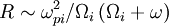 and
and 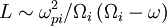 .
The dispersion relation is then (for both Alfvén waves, combined):
.
The dispersion relation is then (for both Alfvén waves, combined):
The Alfvén resonance occurs at  .
.
Lower Hybrid Waves
The lower hybrid wave may be derived using the electrostatic approximation in the lower hybrid frequency range Failed to parse (PNG conversion failed; check for correct installation of latex, dvips, gs, and convert): (\Omega_{i}\ll\omega\ll\Omega_{e}) . The X-mode is affected by the lower hybrid resonance, which occurs at Failed to parse (PNG conversion failed; check for correct installation of latex, dvips, gs, and convert): \omega_{LH}
defined by:
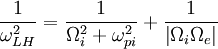
At the frequency  , the minor
diameter of the electron trajectory is equal to the major diameter
of the ion trajectory, and this is the source of the resonance.
, the minor
diameter of the electron trajectory is equal to the major diameter
of the ion trajectory, and this is the source of the resonance.
Quasi-Transverse (QT) Waves
This is a general term for electromagnetic waves propagating approximately
perpendicular to the \emph{magnetic} field (counter to nomenclature),
with Failed to parse (PNG conversion failed; check for correct installation of latex, dvips, gs, and convert): \omega\gg\Omega_{i},\omega_{pi}
,  . There are two
QT modes. The QT-O mode is:
. There are two
QT modes. The QT-O mode is:
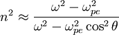
Then for perpendicular (Failed to parse (PNG conversion failed; check for correct installation of latex, dvips, gs, and convert): \theta=\pi/2
) propagation, this wave corresponds
to Failed to parse (PNG conversion failed; check for correct installation of latex, dvips, gs, and convert): n^{2}=P
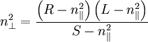
. The QT-X mode is:
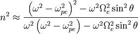
For Failed to parse (PNG conversion failed; check for correct installation of latex, dvips, gs, and convert): \theta=\pi/2
, this wave corresponds to Failed to parse (PNG conversion failed; check for correct installation of latex, dvips, gs, and convert): n^{2}=RL/S
.
Quasi-Longitudinal (QL) Waves (Electron Cyclotron and Whistler Waves)
This is a general term for electromagnetic waves propagating approximately
parallel to the magnetic field (counter to nomenclature), with Failed to parse (PNG conversion failed; check for correct installation of latex, dvips, gs, and convert): \omega\gg\Omega_{i}
,
Failed to parse (PNG conversion failed; check for correct installation of latex, dvips, gs, and convert): \omega_{pi}
, . One may find:
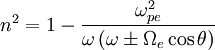
Where the QL-R wave corresponds to the positive sign, and the QL-L
wave corresponds to the negative sign. The QL-R wave is sometimes
known as the whistler wave because the group velocity increases with
frequency. The QL-R wave is sometimes also referred to as the electron
cyclotron wave, due to the resonance at the electron cyclotron frequency.
Upper Hybrid Waves
The upper hybrid wave dispersion relation may be found by using the electrostatic approximation in this regime. The X-mode is affected by the upper hybrid resonance, Failed to parse (PNG conversion failed; check for correct installation of latex, dvips, gs, and convert): \omega_{UH}
defined by:
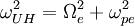
This may be described as the frequency at which electrons on a flux
tube boundary would oscillate if they were all simultaneously displaced
outward.
Warm plasma waves
Ion Acoustic Wave
The ion acoustic wave is analagous to the cold plasma Failed to parse (PNG conversion failed; check for correct installation of latex, dvips, gs, and convert): P=0
wave.
Therefore, we set Failed to parse (PNG conversion failed; check for correct installation of latex, dvips, gs, and convert): \epsilon_{zz}=0 , and find:
Here κ is Boltzmann's constant. These will be strongly damped
by Landau damping unless  ,
which then gives the relation Failed to parse (PNG conversion failed; check for correct installation of latex, dvips, gs, and convert): \omega^{2}=k_{\|}^{2}c_{s}^{2}
.
,
which then gives the relation Failed to parse (PNG conversion failed; check for correct installation of latex, dvips, gs, and convert): \omega^{2}=k_{\|}^{2}c_{s}^{2}
.
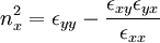
Electrostatic Ion Cyclotron Wave
If we use the electrostatic approximation, and assume Failed to parse (PNG conversion failed; check for correct installation of latex, dvips, gs, and convert): \omega\ll\Omega_{e}<math>, allowing finite <math>k_{x}
and including warm plasma effects, we find
the dispersion relation:
Failed to parse (PNG conversion failed; check for correct installation of latex, dvips, gs, and convert): \omega^{2}=\Omega_{i}^{2}+k_{x}^{2}c_{s}^{2}
Lower-Hybrid Waves
The lower hybrid waves assume Failed to parse (PNG conversion failed; check for correct installation of latex, dvips, gs, and convert): \Omega_{i}<\omega\ll\Omega_{e} . If we include warm plasma effects and density gradients, we get the dispersion relation:

Drift Waves
Drift waves are low frequency electrostatic waves. They arise in inhomogenous
(Failed to parse (PNG conversion failed; check for correct installation of latex, dvips, gs, and convert): n=n
),  ) plasmas with finite parallel electron
temperature. The two possibilities are adiabatic:
) plasmas with finite parallel electron
temperature. The two possibilities are adiabatic:
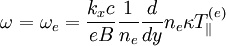
And isothermal:
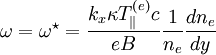
Where the isothermal law is usually the relevant one (it is relevant
assuming  ).
).
Hot Plasma Waves
Ion Cyclotron Waves
In the hot plasma regime, the ion cyclotron wave dispersion relation (also describing the shear Alfvén wave) may be written as:
![n_{\|}^{2}=1-\frac{\omega_{pi}^{2}}{\omega\Omega_{i}}+\left[\frac{\omega_{p}^{2}}{\omega k_{\|}w}Z_{0}\left(\zeta_{1}\right)\right]_{i}](../../images/math/b/4/8/b486101bcbfee6392fea86b46bf0eb24.png)
Note that since 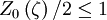 for real ζ,
there is a maximum value for
for real ζ,
there is a maximum value for  .
.
Magnetosonic Waves
These waves correspond to the fast Alfvén wave, so .
The dispersion relation is:
Electron Cyclotron Waves
In the hot plasma regime, the electron cyclotron wave (or QL-L) dispersion relation may be written as:
![n_{\|}^{2}=1-\frac{\omega_{pi}^{2}}{\omega^{2}}+\left[\frac{\omega_{p}^{2}}{\omega k_{\|}w}Z_{0}\left(\zeta_{-1}\right)\right]_{e}](../../images/math/c/b/2/cb2decd954abd1b44a0fdd431ec43b80.png)
Note that since for real ζ,
there is a maximum value for .
Nonresonant Perpendicular Waves
Assuming  and
and  , we find two dispersion
relations corresponding to QT-O waves (Failed to parse (PNG conversion failed; check for correct installation of latex, dvips, gs, and convert): n^{2}=P
):
, we find two dispersion
relations corresponding to QT-O waves (Failed to parse (PNG conversion failed; check for correct installation of latex, dvips, gs, and convert): n^{2}=P
):

which are electromagnetic, and QT-X waves 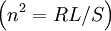 :
:
These waves are approximately electrostatic. \emph{Bernstein waves}
are a subclass of these QT-X waves.
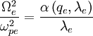
Bernstein Waves}
To derive these waves, it is necessary that and Failed to parse (PNG conversion failed; check for correct installation of latex, dvips, gs, and convert): V=0
.
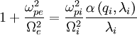
Bernstein waves are electrostatic waves that are cut off near (just
below) the cyclotron harmonics. The dispersion relation is given by:
Failed to parse (PNG conversion failed; check for correct installation of latex, dvips, gs, and convert): \epsilon_{xx}=1-\sum_{s}\frac{4\pi n_{s}m_{s}c^{2}}{B_{0}^{2}}\frac{\alpha\left(q_{s},\lambda_{s}\right)}{\lambda_{s}}=0,\;\alpha\left(q,\lambda\right)=2\sum_{n=1}^{\infty}e^{-\lambda}I_{n}\left(\lambda\right)\frac{n^{2}}{q^{2}-n^{2}}
with Failed to parse (PNG conversion failed; check for correct installation of latex, dvips, gs, and convert): q=\omega/\Omega . For frequencies well above Failed to parse (PNG conversion failed; check for correct installation of latex, dvips, gs, and convert): \Omega_{i} , we have approximately the \emph{electron Bernstein mode}, with dispersion relation:
while for frequencies well below Failed to parse (PNG conversion failed; check for correct installation of latex, dvips, gs, and convert): \Omega_{e}
, the wave describes
an \emph{ion Bernstein mode}, with dispersion relation:
Instabilities
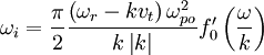
Landau Damping
Landau damping occurs for Failed to parse (PNG conversion failed; check for correct installation of latex, dvips, gs, and convert): \omega\sim vt
for some species. It is
valid in the collisional regime where Failed to parse (PNG conversion failed; check for correct installation of latex, dvips, gs, and convert): \nu_{coll}\tau_{osc}>1
and
Failed to parse (PNG conversion failed; check for correct installation of latex, dvips, gs, and convert): k_{\|}\lambda_{mfp}<1 . The collision time is greater than the oscillation time in the electrostatic well (therefore, particles can be considered uncorrelated). The relevant wavelength must be less than the mean free path (so that the plasma is not considered truly collisional). The dispersion relation is:
Assuming  .
.
Two-Stream Instability
This instability occurs for two-peaked energy distributions, beam species, or fast particles. The condition for instability is that:
Failed to parse (PNG conversion failed; check for correct installation of latex, dvips, gs, and convert): \frac{\mathbf{k}\cdot\left(\mathbf{v}_{1}-\mathbf{v}_{2}\right)}{2\omega_{po}}<1
Where 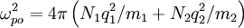 .
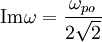
The fastest growing mode corresponds to Failed to parse (PNG conversion failed; check for correct installation of latex, dvips, gs, and convert): x^{2}=3/8
.
The fastest growing mode corresponds to Failed to parse (PNG conversion failed; check for correct installation of latex, dvips, gs, and convert): x^{2}=3/8
and has growth
rate:
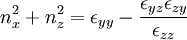
Rayleigh-Taylor Instability
This instability occurs when the magnetic field, acting as a light
fluid, must accelerate a heavy fluid, the plasma. This an the instability
that grows, for example, in bad curvature regions. The dispersion
relation in the case that 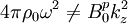 (p superscripts indicate values in the plasma, v superscripts
indicate values in the vacuum):
(p superscripts indicate values in the plasma, v superscripts
indicate values in the vacuum):
![\omega^{2}=\frac{1}{4\pi\rho_{0}}\left[\left(\mathbf{B}_{0}^{p}\cdot\mathbf{k}\right)^{2}+\left(\mathbf{B}_{0}^{v}\cdot\mathbf{k}\right)^{2}\right]-g\left(k_{x}^{2}+k_{z}^{2}\right)^{1/2}](../../images/math/4/1/b/41b3cf86cddd61c1c6d6d1511489f818.png)
where  , so that this will
be unstable anywhere
, so that this will
be unstable anywhere  . The case
that
. The case
that 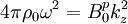 is stable and damped
in Failed to parse (PNG conversion failed; check for correct installation of latex, dvips, gs, and convert): k_{y}
.
is stable and damped
in Failed to parse (PNG conversion failed; check for correct installation of latex, dvips, gs, and convert): k_{y}
.
Transit-Time Damping
Transit-time damping is the magnetic analog to Landau damping. It
comes from the interaction of the magnetic moment of a gyrating particle,
\textgreek{m}, with a parallel magnetic field gradient. Because the
resonance condition is the same as the Landau damping ( ),
there may be either constructive or destructive coherence between
the two processes.
),
there may be either constructive or destructive coherence between
the two processes.
Fire-Hose Instability
The fire-hose instability arises from the hot plasma shear Alfvén wave. The instability condition is that:
Failed to parse (PNG conversion failed; check for correct installation of latex, dvips, gs, and convert): \beta_{\|}>\beta_{\perp}+2
with 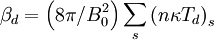 .
One may think of it as:
.
One may think of it as:
Failed to parse (PNG conversion failed; check for correct installation of latex, dvips, gs, and convert): p_{\|}>p_{\perp}+\frac{B_{0}^{2}}{4\pi}
The instability occurs when deviations in the field line direction cause the parallel pressure to oppose the perpendicular pressure. If it is stronger, it stretches the field lines and the instability grows.
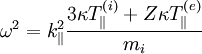
Magnetosonic Instability
The magnetosonic instability arises from the magnetosonic move (compressional Alfvén wave). In the case that Failed to parse (PNG conversion failed; check for correct installation of latex, dvips, gs, and convert): \left(T_{\parallel}/T_{\perp}\right)_{i}=\left(T_{\|}/T_{\perp}\right)_{e} , the instability condition is that:
Failed to parse (PNG conversion failed; check for correct installation of latex, dvips, gs, and convert): \frac{\beta_\perp^{2}}{\beta_\parallel} > 1+\beta_\perp
This is a pressure-anisotropy driven instability.


