M3D-C1
Reference Documents User's Guide Tutorial Model Reference Release Notes IDL Reference Normalization Spreadsheet
Introduction
M3D-C1 is a code that solves the extended-magnetohydrodynamic (MHD) equations, which is a model that describes plasma as electrically conducting fluids of ions and electrons. This code is primarily used for calculating the equilibrium, stability, and dynamics of fusion plasmas, but has also been used for a variety of other applications, including astrophysical applications. In particular, M3D-C1 is designed to address some of the most critical challenges confronting tokamak plasmas: large-scale instabilities, which significantly degrade thermal confinement; and disruptions, which cause complete loss of energy confinement and which may cause damage to reactor-scale tokamaks such as ITER.
M3D-C1 builds upon some of the design principles pioneered by M3D, but the two codes are developed independently and do not share source code. The "C1" in M3D-C1 refers to the $C^1$ property of its finite elements, which ensures that both the value and the derivatives of fields are continuous across mesh element boundaries.
Advanced numerical methods are employed in M3D-C1 to permit the efficient solution of its numerical model over a broad range of temporal and spatial scales. These methods include the use of high-order finite elements on an unstructured mesh; fully implicit and semi-implicit time integration options; physics-based preconditioning; and parallelization via domain decomposition and the use of scalable parallel sparse linear algebra solvers.
Documents describing how to use and run the code, and publications describing the numerical methods and physics results in more detail, can be found in the reference documents and the bibliography below.
Applications
Vertical Displacement Events (VDEs)
|
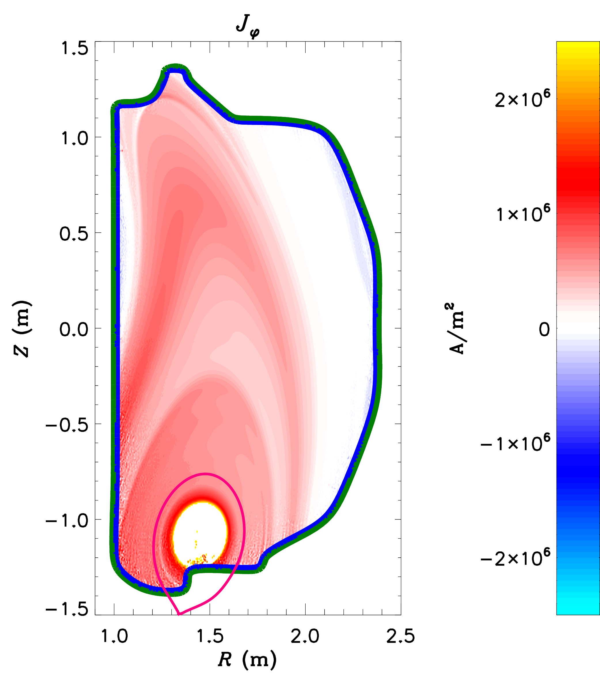
Vertical Displacement Events (VDEs) are disruptions that occur when the vertical control of a tokamak plasma is lost, and the plasma rapidly moves upward or downward into the inner walls of the confinement vessel. These events not only terminate the plasma discharge, but may cause enormous heat loads and electromagnetic stresses on the vessel. M3D-C1 is being used to characterize these instabilities, to gain insight into the location and magnitude of the expected heat loads and thermal stresses. The resistive wall model in M3D-C1 allows the modeling of "Halo currents," which are electrical currents that flow from the plasma to the wall and back. These currents are thought to be responsible for a significant fraction of the electromagnetic forces on the vessel during a disruption. |
|
A description of 2D VDE calculations with M3D-C1 is given in NM Ferraro, et al. Phys. Plasmas 23:056114 (2016).
Sawteeth and Helical Core Equilibria
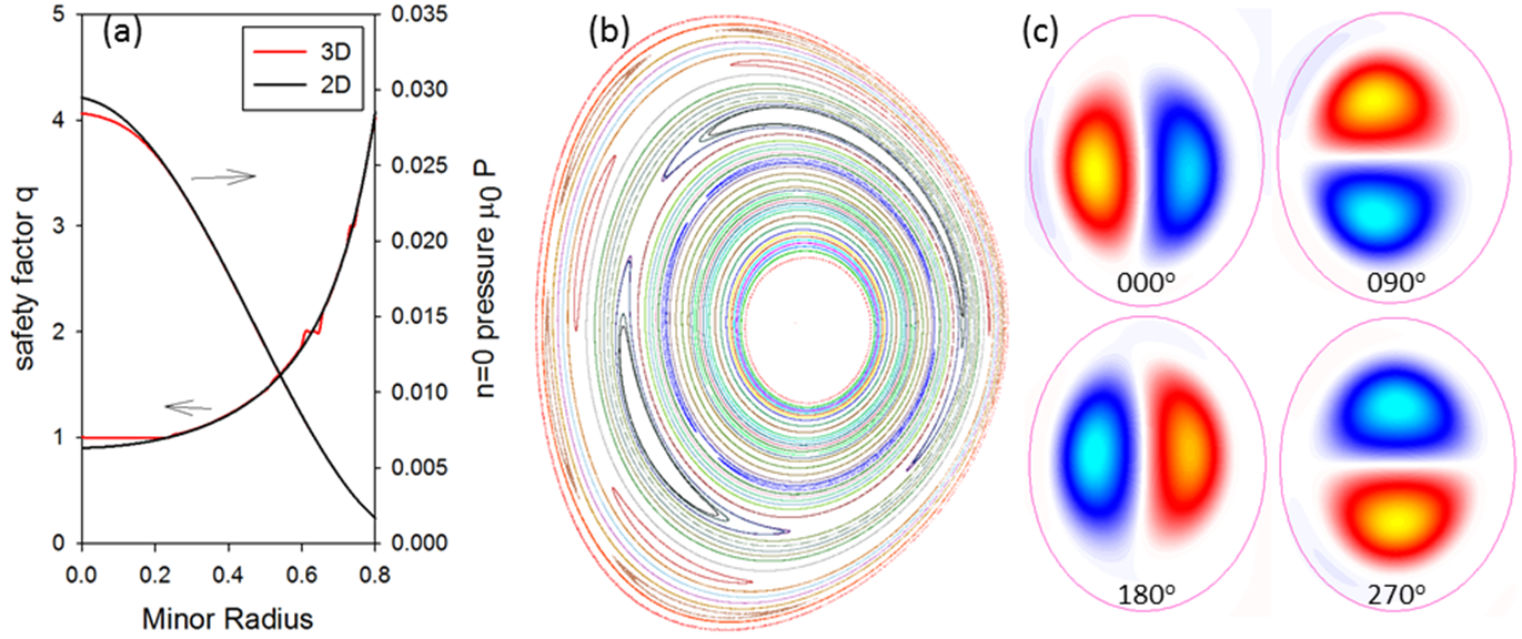 (a) $q$-profile and toroidally-averaged $p$ for 3D run, and 2D
run with the same transport coefficients.
(a) $q$-profile and toroidally-averaged $p$ for 3D run, and 2D
run with the same transport coefficients.
(b) Poincare
plot in the final state with $(2, 1)$ and $(3, 1)$ islands
present (central volume has $q=1$).
(c) Contours of
electrostatic potential, $\phi$, produced by the stationary
interchange mode.
In most tokamak discharges, the plasma current slowly peaks until it becomes unstable to internal kink modes. This so-called "sawtooth" instability flattens the central current; at which time the process repeats. While these oscillations are generally benign, they are likely best avoided in burning plasmas: high-energy fusion products ($\alpha$-particles) can increase the oscillation amplitude, which may excite neoclassical tearing modes and/or edge localized modes, potentially causing major disruptions. Using the M3D-C1 code another mechanism for preventing the current from peaking that involves a self-organized, dynamo action was found, which avoids these problems.
Numerical simulations and analytic theory have determined that, for certain, global parameters, the plasma will self-organize with the central safety-factor, $q$, slightly above unity and constant in a central volume (as shown in above figure, click to enlarge), where $q$ is defined as how many times a magnetic field line travels around the torus the long way compared to the short way. Such a large, "shear"-free region is unstable to pressure-driven "interchange" modes. The linearly-unstable, interchange eigenfunction extends throughout the shear-free region and drives a strong, stationary, $(1,1)$-helical flow that then drives a stationary $(1,1)$-component of the electrostatic potential, $\phi$, (shown) and of the magnetic field (shown). These combine to create a $(0,0)$-"dynamo" voltage that prevents the current density from peaking in the center, hence maintaining the shear-free region with $q$ slightly above unity in the central region, and with a broad current profile. This mechanism could explain the physics behind the non-sawtoothing "hybrid" discharges observed in DIII-D and in many other tokamaks.
For more details, see SC Jardin, N Ferraro, I Krebs. Phys. Rev. Lett. 115:215001 (2015).
Edge-Localized Modes (ELMs)
The high-confinement mode (H-mode) of tokamak plasma operation is characterized by steep thermal gradients and large current densities at the edge of the plasma. While H-mode is advantageous from a confinement standpoint, the large pressure gradients and current densities lead to periodic instabilities known as Edge Localized Modes (ELMs) that intermittently deliver significant heat loads to plasma-facing components of the confinement vessel. In reactor-scale devices like ITER, these heat loads may be large enough to rapidly erode these components, and therefore must be mitigated.
M3D-C1 has been used to calculate how various non-ideal effects, including resistivity, rotation, and two-fluid terms change ELM stability. For example, see NM Ferraro (2010). M3D-C1 has also been used to simulate the nonlinear evolution of ELMs, in order to better understand the thermal transport that these modes cause.
Linear Response to Applied 3D Fields
|
The magnetic fields in tokamaks are nominally axisymmetric (independent of toroidal angle). It has been observed, however, that applying small non-axisymmetric fields to the plasma can have a significant effect on confinement and ELM stability. In particular, ELM suppression through the application of non-axisymmetric fields is one of the primary techniques for mitigating the intermittent heat bursts caused by ELMs. It is not yet understood why applying non-axisymmetric fields sometimes mitigates or suppresses ELMs. Part of the difficulty in understanding this process is that the applied field drives currents in the plasma, which themselves create non-axisymmetric fields. These "plasma response" fields are often stronger than the applied fields themselves. So a challenge in understanding these effects is being able to calculate the plasma response given the applied fields. Developing this understanding is crucial for being able to confidently design coils for this technique on reactor-scale devices. M3D-C1 has been used extensively to calculate the plasma response to applied fields in DIII-D, AUG, NSTX, NSTX-U, KSTAR, and model ITER plasmas. |
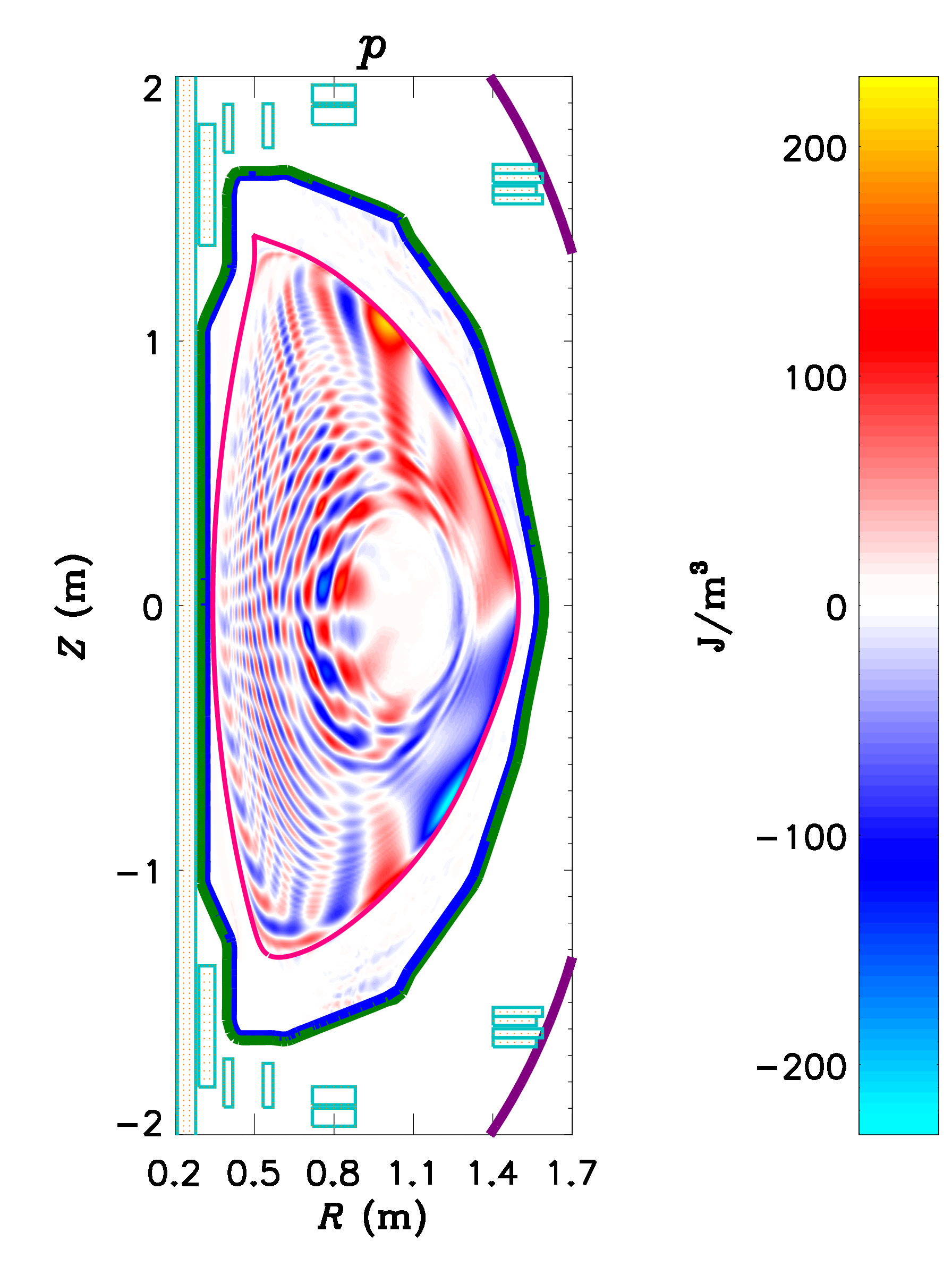 The
pressure perturbations that will be produced by applying
non-axisymmetric fields from the proposed Non-axisymmetric
Control Coils (NCC) to a model NSTX-U equilibrium, as
calculated by M3D-C1. The
pressure perturbations that will be produced by applying
non-axisymmetric fields from the proposed Non-axisymmetric
Control Coils (NCC) to a model NSTX-U equilibrium, as
calculated by M3D-C1.
|
Physical Model
The extended-MHD model implemented in M3D-C1 consists of a set of fluid equations which evolve the particle number density $n$, fluid velocity $\vec{u}$, total pressure $p$, and electron pressure $p_e$: \begin{eqnarray} \frac{\partial n}{\partial t} + \nabla \cdot (n \vec{u}) & = & 0 \\ n m_i \left(\frac{\partial \vec{u}}{\partial t} + \vec{u} \cdot \nabla \vec{u} \right) & = & \vec{J} \times \vec{B} - \nabla p \color{blue}{ \mbox{} - \nabla \cdot \Pi + \vec{F}} \\ \frac{\partial p}{\partial t} + \vec{u} \cdot \nabla p + \Gamma p \nabla \cdot \vec{u} & = & \color{blue}{(\Gamma - 1) \left[Q - \nabla \cdot \vec{q} + \eta J^2 - \vec{u} \cdot \vec{F} - \Pi : \nabla u \right]} \\ & & \color{red}{\mbox{} + \frac{1}{n e} \vec{J} \cdot \left( \frac{\nabla n}{n} p_e - \nabla p_e \right) + (\Gamma-1) \Pi_e : \nabla \left(\frac{1}{n e} \vec{J} \right)} \\ \frac{\partial p_e}{\partial t} + \vec{u} \cdot \nabla p_e + \Gamma p_e \nabla \cdot \vec{u} & = & \color{blue}{(\Gamma - 1) \left[Q_e - \vec{q}_e + \eta J^2 - \vec{u} \cdot \vec{F}_e - \Pi_e : \nabla u \right]} \\ & & \color{red}{\mbox{} + \frac{1}{n e} \vec{J} \cdot \left( \frac{\nabla n}{n} p_e - \nabla p_e \right) + (\Gamma-1) \left[ \Pi_e : \nabla \left(\frac{1}{n e} \vec{J} \right) + \frac{1}{n e} \vec{J} \cdot \vec{F}_e \right]} \end{eqnarray} a generalized Ohm's law, in which the electric field $\vec{E}$ is obtained from the equations describing conservation of electron momentum and charge: \begin{equation} \vec{E} = - \vec{u} \times \vec{B} \color{blue}{ \mbox{} +\eta \vec{J}} \color{red}{ \mbox{} + \frac{1}{n e} \left( \vec{J} \times \vec{B} - \nabla p_e - \nabla \cdot \Pi_e + \vec{F}_e \right)} \end{equation} and a reduced set of Maxwell's equations which relates the electrical current density $\vec{J}$ in the plasma to the magnetic field $\vec{B}$ and describes the evolution of the magnetic field: \begin{eqnarray} \vec{J} & = & \frac{1}{\mu_0} \nabla \times \vec{B} \\ \frac{\partial \vec{B}}{\partial t} & = & -\nabla \times \vec{E} \end{eqnarray}
The "Ideal-MHD" model is a subset of the one described above, which is obtained in the limit where external sources, dissipative terms (like viscosity and resistivity) and the ion Larmor radius are zero, leaving only the terms colored black. "Single-Fluid MHD" is a larger subset, in which the ions and electrons are considered to have the same fluid velocity and temperature, but where dissipative terms and external sources are included, shown in blue. M3D-C1 implements a "Two-Fluid" model, which takes differences in the ion and electron fluid velocities into account, which introduces the terms colored red. M3D-C1 may also be used for solving the single-fluid equations. The ideal-MHD equations are best solved using specialized codes such as DCON, IPEC, GATO, ELITE, VMEC, or SPEC, which are designed to take advantage of special properties of the ideal-MHD equations.
$\vec{F} = \vec{F}_i + \vec{F}_e$, where $\vec{F}_i$ and $\vec{F}_e$ are external forces acting on the ions and electrons, respectively (e.g. gravity). Similarly, $Q = Q_i + Q_e$, where $Q_i$ and $Q_e$ are external sources of heat to the ions and electrons. In M3D-C1, several processes are implemented that are represented by these sources, including neutral beam injection.
The viscous stress tensor $\Pi = \Pi_i + \Pi_e$ is the sum of the ion and electron stress tensors. Several processes contributing to the ion stress tensor are implemented: \begin{equation} \Pi_i = \Pi_i^\perp + \Pi_i^\wedge + \Pi_i^\parallel \end{equation} where $\Pi_i^\perp$ is the perpendicular ion viscosity, which represents simple cross-field angular momentum diffusivity; $\Pi_i^\wedge$ is the ion gyroviscosity, which represents finite ion Larmor radius effects; and $\Pi_i^\parallel$ is the parallel ion viscosity, which represents pressure anisotropy and is responsible for ion sound wave damping and poloidal flow damping in the extended-MHD model. Presently, the $\Pi_e$ term is implemented as a hyper-resistive term.
The heat flux density $\vec{q} = \vec{q}_i + \vec{q}_e$ is the sum of the ion and electron heat flux densities, which themselves are represented as the sum of perpendicular and parallel parts: \begin{equation} \vec{q}_{(i,e)} = -\kappa_{(i,e)}^\perp \nabla T_{(i,e)} - \kappa_{(i,e)}^\parallel \frac{\vec{B} \vec{B} \cdot \nabla T_{(i,e)}}{B^2} \end{equation}
M3D-C1's equations are formulated in $(R,\varphi,Z)$ coordinates, and do not make use of magnetic coordinates. Therefore there is no coordinate singularity at poloidal field nulls (such as the magnetic axis or x-points of toroidal plasmas), and no need to impose boundary conditions there.
The model implemented in M3D-C1 contains far more options than can be reasonably described here. For a more detailed, complete, and up-to-date description of the model implemented in M3D-C1, please refer to the M3D-C1 Model Reference.
Reduced Models
A useful feature of M3D-C1 is that it represents the magnetic field and fluid velocity using stream functions and potentials, similar to a Helmholtz decomposition: \begin{eqnarray} \vec{B} & = & \nabla \psi \times \nabla \varphi + F \nabla \varphi \\ \vec{u} & = & R^2 \nabla U \times \nabla \varphi + R^2 \omega \nabla \varphi + R^{-2} \nabla_\perp \chi \end{eqnarray}
One advantage of this representation is that the magnetic field is manifestly divergence-free. Another advantage is that we obtain physically meaningful reduced models by restricting the set of scalar fields that are evolved. Specifically, we obtain the two-field reduced model by only considering the evolution of $\psi$ and $U$, and we obtain the four-field reduced model by only considering the evolution of $\psi$, $U$, $F$, and $\omega$. These reduced models provide accurate solutions in certain physical limits, at a fraction of the computational cost of the full extended-MHD model.
Resistive Wall
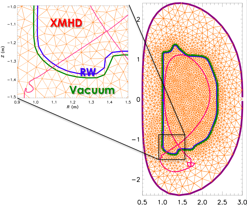
M3D-C1 optionally includes a resistive wall model, which is treated as a spatially resolved region of arbitrary thickness. This capability enables the study of so-called "resistive wall modes" (RWMs) in tokamaks, which are external kink modes that would be stable in the presence of a perfectly conducting wall, but which are unstable when the wall has finite resistivity.
|
In calculations that include a resistive wall, the computational domain is divided into three parts. The innermost part is the extended-MHD (XMHD) region, in which the full extended-MHD model is solved. Enclosing this region is the resistive wall (RW) region, in which only Maxwell's equations are solved, with $\vec{E} = \eta_w \vec{J}$. Enclosing this region is the vacuum region, where only $\eta{J} = 0$ is solved. The equations in these regions are solved self-consistently and simultaneously, using implicit time-stepping methods. |
Numerical Methods
Finite Elements
In its 2D and 2D-complex modes of operation, M3D-C1 uses two-dimensional, reduced-quintic triangular finite elements on an unstructured mesh. These high-order, $C^1$ elements are described in detail in SC Jardin J. Comp. Phys. 200:133 (2004).
In its 3D mode of operation, M3D-C1 uses three-dimensional triangular-prism elements that are a tensor product of the triangular reduced-quintic elements in the poloidal plane with cubic Hermite elements in the toroidal (or axial) direction. These three-dimensional elements also have the $C^1$ property.
Implicit and Semi-Implicit Time Advance
Reference Documents
- User's Guide: Comprehensive reference that covers building and running M3D-C1, mesh generation, example problems, and descriptions of the input files.
- Model Reference: A description of the physics model implemented in M3D-C1 and the input parameters controlling the model.
- Tutorial: A short reference guide describing running the code for some common use cases.
- IDL Reference: A description of the IDL visualization and post-processing routines provided with M3D-C1
- Release Notes: A list of new features in each release of M3D-C1
- Normalization Spreadsheet: A spreadsheet for translating between M3D-C1 normalized units and physical units
How to Obtain M3D-C1
To run or obtain the source code for M3D-C1 please complete and submit the PPPL Theory Codes License-Release form. Please note that this agreement requires that a designee of PPPL be allowed to review any output of M3D-C1 prior to publication to help ensure that the code has been run correctly and that the results have been properly interpreted.
Acknowledgments
The development of M3D-C1 has been supported by the US Department of Energy through the Center for Extended MHD Modeling (CEMM) and Center for Tokamak Transient Simulations (CTTS) SciDAC activities. The numerical tools and methods relating to meshing and domain decomposition are developed through a collaboration with the RPI SCOREC group.
Publications
The following is a list of publications that focus primarily on M3D-C1 modeling or numerical methods. It does not include publications that feature M3D-C1 calculations in support of understanding specific experiments.
If you would like to cite M3D-C1, please see the list of references by subject to find the best appropriate references.
- BC Lyons, CC Kim, YQ Liu, NM Ferraro, SC Jardin, J McClenaghan, PB Parks, LL Lao. "Axisymmetric benchmarks of impurity dynamics in extended-magnetohydrodynamic simulations." Plasma Phys. Control. Fusion 61:064001 (2019)
- NM Ferraro, BC Lyons, CC Kim, YQ Liu, and SC Jardin. "3D two-temperature magnetohydrodynamic modeling of fast thermal quenches due to injected impurities in tokamaks." Nucl. Fusion 59:016001 (2019)
- D Pfefferle, N Ferraro, SC Jardin, I Krebs, and A Bhattacharjee. "Modelling of NSTX hot vertical displacement events using M3D-C1." Phys. Plasmas 25:056106 (2018)
- NM Ferraro, SC Jardin, LL Lao, MS Shephard, F Zhang. "Multi-region approach to free-boundary three-dimensional tokamak equilibria and resistive wall instabilities." Phys. Plasmas 23:056114 (2016)
- F Zhang, R Hager, S-H Ku, C-S Chang, SC Jardin, NM Ferraro, S Seol, E Yoon, MS Shephard. "Mesh generation for confined fusion plasma simulation." Engineering with Computers p. 1–9 (2015)
- NM Ferraro. "Calculations of two-fluid linear response to non-axisymmetric fields in tokamaks." Phys. Plasmas 19:056105 (2012)
- SC Jardin, N Ferraro, J Breslau, J Chen. "Multiple timescale calculations of sawteeth and other global macroscopic dynamics of tokamak plasmas." Comp. Sci. & Disc. 5:014002 (2012)
- NM Ferraro, SC Jardin, PB Snyder. "Ideal and resistive edge stability calculations with M3D-C1." Phys. Plasmas 17:102508 (2010)
- NM Ferraro, SC Jardin. "Calculations of two-fluid magnetohydrodynamic axisymmetric steady-states." J. Comp. Phys. 228:7742 (2009)
- J Breslau, N Ferraro, S Jardin. "Some properties of the M3D-C1 form of the three-dimensional magnetohydrodynamics equations." Phys. Plasmas 16:092503 (2009)
- SC Jardin, N Ferraro, X Luo, J Chen, J Breslau, KE Jansen, MS Shephard. "The M3D-C1 approach to simulating 3D 2-fluid magnetohydrodynamics in magnetic fusion experiments." J. Phys.: Conf. Series 125:012044 (2008)
- SC Jardin, J Breslau, N Ferraro. "A high-order implicit finite element method for integrating the two-fluid magnetohydrodynamic equations in two dimensions." J. Comp. Phys. 226:2146 (2007)
- NM Ferraro and SC Jardin. "Finite element implementation of Braginskii's gyroviscous stress with application to the gravitational instability." Phys. Plasmas 13:092101 (2006)
- SC Jardin. "A triangular finite element with first-derivative continuity applied to fusion MHD applications." J. Comp. Phys. 200:133 (2004)
References By Subject
The following list includes some of the best references for the implementation of various models in M3D-C1, as well as some references to the application of the code to physical phenomena.
- Disruption Mitigation: Ferraro 2019, Lyons 2019, Fil 2017
- Edge Localized Modes Ferraro 2010, Wingen 2015
- Impurity Model: Ferraro 2019
- MHD Model: Breslau 2009
- Non-axisymmetric Tokamak Equilibria (nonlinear): Jardin 2015, Krebs 2017, Reiman 2015
- Pellet Model: Lyons 2019
- Perturbed Tokamak Equilibria (linear): Ferraro 2012, Ferraro 2013, Lyons 2017, Canal 2017, Wingen 2015, Reiman 2015
- Resistive Wall Model: Ferraro 2016
- Resistive Wall Modes: Ferraro 2016
- Sawteeth: Jardin 2015, Jardin 2012
- Vertical Displacement Events: Pferrerle 2018, Ferraro 2016