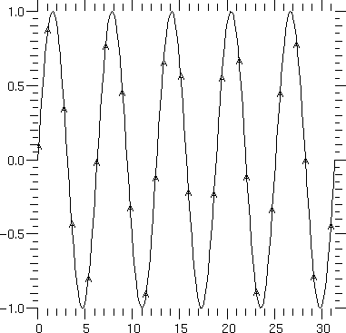
The following draws the graph of a sine curve:

Plot a graph of y versus x. y and x must be 1-D arrays of equal length. If x is omitted, it defaults to [1, 2, ..., len(y)].
The following keyword argument(s) apply only to this function.
rspace = <float value>
rphase = <float value>
arroww = <float value>
arrowl = <float value>
Select the spacing, phase, and size of occasional ray arrows placed along polylines. The spacing and phase are in NDC units (0.0013 NDC equals 1.0 point); the default rspace is 0.13, and the default rphase is 0.11375, but rphase is automatically incremented for successive curves on a single plot. The arrowhead width, arroww, and arrowhead length, arrowl are in relative units, defaulting to 1.0, which translates to an arrowhead 10 points long and 4 points in half-width.
The following additional keyword arguments can be specified with this function.
legend, hide, type, width, color, closed, smooth, marks, marker, mspace, mphase, rays
See "Plot Function Keywords" on page 45 for detailed descriptions of these keywords.
The following example simply plots two straight lines..
The following draws the graph of a sine curve:

Set the default mesh for subsequent plm, plc, plv, plf, and plfc calls. In the second form, plmesh deletes the default mesh (until you do this, or switch to a new default mesh, the default mesh arrays persist and takes up space in memory). The y, x, and ireg arrays should all be the same shape; y and x will be converted to double, and ireg will be converted to int.
If ireg is omitted, it defaults to ireg(0,)=ireg(,0)=0, ireg(1:,1:)=1; that is, region number 1 is the whole mesh. The triangulation array tri_array is used by plc and plfc; the correspondence between tri_array indices and zone indices is the same as for ireg, and its default value is all zero. The ireg or tri_array arguments may be supplied without y and x to change the region numbering or triangulation for a given set of mesh coordinates. However, a default y and x must already have been defined if you do this. If y is supplied, x must be supplied, and vice-versa.
The following example creates a mesh whose graph we will see later (see the example on page 31). For convenience, we show the functions span and a3, which are used to build the data.
Plot a mesh of y versus x. y and x must be 2-D arrays with equal dimensions. If present, ireg must be a 2-D region number array for the mesh, with the same dimensions as x and y. The values of ireg should be positive region numbers, and zero for zones which do not exist. The first row and column of ireg never correspond to any zone, and should always be zero. The default ireg is 1 everywhere else.
The y, x, and ireg arguments may all be omitted to default to the mesh set by the most recent plmesh call.
The following keyword argument(s) apply only to this function.
If present, the boundary keyword determines whether the entire mesh is to be plotted (boundary=0, the default), or just the boundary of the selected region (boundary=1).
If present, the inhibit keyword causes the (x(,j),y(,j)) lines to not be plotted (inhibit=1), the (x(i,),y(i,)) lines to not be plotted (inhibit=2), or both sets of lines not to be plotted (inhibit=3). By default (inhibit=0), mesh lines in both logical directions are plotted.
The following additional keyword arguments can be specified with this function.
legend, hide, type, width, color, region
See "Plot Function Keywords" on page 45 for detailed descriptions of these keywords.
The mesh set by the plmesh function call in the preceding example (page 30) may be plotted simply by calling plm with no arguments:
Plot contours of z on the mesh y versus x. y, x, and ireg are as for plm. The z array must have the same shape as y and x. The function being contoured takes the value z at each point (x,y); that is, the z array is presumed to be point-centered. The y, x, and ireg arguments may all be omitted to default to the mesh set by the most recent plmesh call.
The following keyword argument(s) apply only to this function.
The levs keyword specifies a list of the values of z at which you want contour curves. The default is eight contours spanning the range of z.
Set the triangulation array for a contour plot. triangle must be the same shape as the ireg (region number) array, and the correspondence between mesh zones and indices is the same as for ireg. The triangulation array is used to resolve the ambiguity in saddle zones, in which the function z being contoured has two diagonally opposite corners high, and the other two corners low. The triangulation array element for a zone is 0 if the algorithm is to choose a triangulation, based on the curvature of the first contour to enter the zone. If zone (i,j) is to be triangulated from point (i-1,j-1) to point (i,j), then triangle(i,j)=1, while if it is to be triangulated from (i-1,j) to (i,j-1), then triangle(i,j)=-1. Contours will never cross this ``triangulation line''.
You should rarely need to fiddle with the triangulation array; it is a hedge for dealing with pathological cases.
The following additional keyword arguments can be specified with this function.
legend, hide, type, width, color, smooth, marks, marker, mspace, mphase, region
See "Plot Function Keywords" on page 45 for detailed descriptions of these keywords.
The following example gives a contour plot of the same mesh used in the preceding two examples. Calling plm with boundary = 1 and region = 1 plots the boundary of the mesh (which, by default, is one region); then calling plc plots a default number of contours (8).
Plot a vector field (vx,vy) on the mesh (x,y). y, x, and ireg are as for plm. The vy and vx arrays must have the same shape as y and x. The y, x, and ireg arguments may all be omitted to default to the mesh set by the most recent plmesh call.
The following keyword argument(s) apply only to this function.
The scale keyword is the conversion factor from the units of (vx,vy) to the units of (x,y) -- a time interval if (vx,vy) is a velocity and (x,y) is a position -- which determines the length of the vector "darts" plotted at the (x,y) points.
If omitted, scale is chosen so that the longest ray arrows have a length comparable to a "typical" zone size. You can use the scalem keyword in pledit to make adjustments to the scale factor computed by default.
hollow = 0/1
aspect = <float value>
Set the appearance of the "darts" of a vector field plot. The default darts, hollow=0, are filled; use hollow=1 to get just the dart outlines. The default is aspect=0.125; aspect is the ratio of the half-width to the length of the darts. Use the color keyword to control the color of the darts.
The following additional keyword arguments can be specified with this function.
legend, hide, type, width, color, smooth, marks, marker, mspace, mphase, triangle, region
See "Plot Function Keywords" on page 45 for detailed descriptions of these keywords.
This example applies to the same mesh that we have considered in the last three examples.
Plot a filled mesh y versus x. y, x, and ireg are as for plm. The z array must have the same shape as y and x, or one smaller in both dimensions. If z is of type unsigned char (Python typecode 'b'), it is used "as is"; otherwise, it is linearly scaled to fill the current palette, as with the bytscl function. The mesh is drawn with each zone in the color derived from the z function and the current palette; thus z is interpreted as a zone-centered array. The y, x, and ireg arguments may all be omitted to default to the mesh set by the most recent plmesh call.
A solid edge can optionally be drawn around each zone by setting the edges keyword non-zero. ecolor and ewidth determine the edge color and width. The mesh is drawn zone by zone in order from ireg(2+imax) to ireg(jmax*imax) (the latter is ireg(imax,jmax)), so you can achieve 3D effects by arranging for this order to coincide with back-to-front order. If z is nil, the mesh zones are filled with the background color, which you can use to produce 3D wire frames.
The following keyword argument(s) apply only to this function.
edges = 0/1
ecolor = <color value>
ewidth = <float value>
Set the appearance of the zone edges in a filled mesh plot (plf). By default, edges=0, and the zone edges are not plotted. If edges=1, a solid line is drawn around each zone after it is filled; the edge color and width are given by ecolor and ewidth, which are "fg" and 1.0 by default.
The following additional keyword arguments can be specified with this function.
legend, hide, region, top, cmin, cmax
See "Plot Function Keywords" on page 45 for detailed descriptions of these keywords. (See the bytscl function description on page 52 for explanation of top, cmin, cmax.)
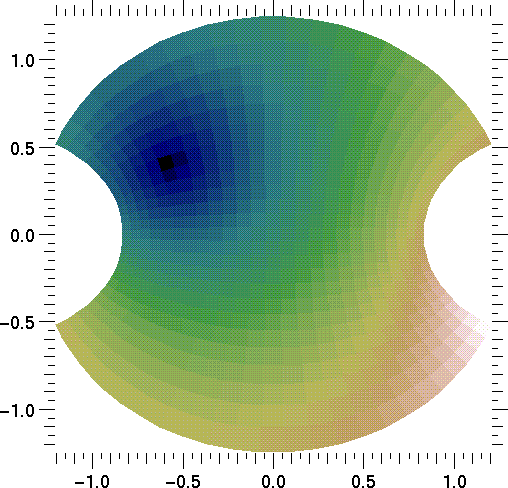
The following gives a filled mesh plot of the same mesh we have been considering in the preceding examples.

Unlike the other plotting primitives, plfc is implemented in Python code. It calls a C module to compute the contours, then uses plfp (described in the next subsection) to draw the filled contour lines. It does not use the mesh plotting routines; hence the arguments z, y, x, and ireg must be given explicitly. They will not default to the values set by plmesh.
The values given above for the keyword arguments are the defaults. The meanings of the keywords are as follows:
If an integer, specifies the number of contour lines desired. The contour levels will be computed automatically. If an array of floats, specifies the actual contour levels.
An array of unsigned char (Python typecode 'b') with values between 0 and 199 specifying the indices into the current palette of the fill colors to use. The size of this array (if present) must be one larger than the number of contours specified.
As described for the mesh plots.
If the number of contours was given, this keyword specifies how they are to be computed: "lin" (linearly), "log" (logarithmically) and "normal" (based on the normal distribution; the minimum and maximum contours will be two standard deviations from the mean).
In the following example, we have to explicitly compute and pass an ireg array. We plot filled contours and then plot contour lines on top of them. Note that the contour divisions do not coincide, since the two routines use different algorithms for computing contour levels. Perhaps someday this defect will be remedied.
Plot a list of filled polygons y versus x, with colors z. The n array is a 1D list of lengths (number of corners) of the polygons; the 1D colors array z has the same length as n. The x and y arrays have length equal to the sum of all dimensions of n.
If z is of type unsigned char (Python typecode "b"), it is used ``as is''; otherwise, it is linearly scaled to fill the current palette, as with the bytscl function.
The following keyword arguments can be specified with this function.
legend, hide, top, cmin, cmax
See "Plot Function Keywords" on page 45 for detailed descriptions of these keywords. (See the bytscl function description on page 52 for explanation of top, cmin, cmax.)
This example gives a sort of "stained glass window" effect;.
Plot the image z as a cell array: an array of equal rectangular cells colored according to the 2-D array z. The first dimension of z is plotted along x, the second dimension is along y.
If z is of type unsigned char (Python typecode "b"), it is used ``as is''; otherwise, it is linearly scaled to fill the current palette, as with the bytscl function.
If x1 and y1 are given, they represent the coordinates of the upper right corner of the image. If x0, and y0 are given, they represent the coordinates of the lower left corner, which is at (0,0) by default. If only the z array is given, each cell will be a 1x1 unit square, with the lower left corner of the image at (0,0).
The following keyword arguments can be specified with this function.
legend, hide, top, cmin, cmax
See "Plot Function Keywords" on page 45 for detailed descriptions of these keywords. (See the bytscl function description on page 52 for explanation of top, cmin, cmax.)
The following example computes and draws an interesting cell array.
Plot disjoint lines from (x0,y0) to (x1,y1). x0, y0, x1, and y1 may have any dimensionality, but all must have the same number of elements.
The following keyword arguments can be specified with this function.
legend, hide, type, width, color
See "Plot Function Keywords" on page 45 for detailed descriptions of these keywords. (See the bytscl function description on page 52 for explanation of top, cmin, cmax.)
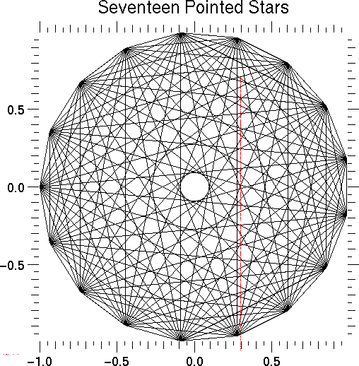
This example draws a set of seventeen-pointed stars.

Plot text (a string) at the point (x,y). The exact relationship between the point (x,y) and the text is determined by the justify keyword. text may contain newline ("\n") characters to output multiple lines of text with a single call.
The coordinates (x,y) are NDC coordinates (outside of any coordinate system) unless the tosys keyword is present and non-zero, in which case the text will be placed in the current coordinate system. However, the character height is never affected by the scale of the coordinate system to which the text belongs.
Note that the pledit command (see "pledit: Change Plotting Properties" on page 49) takes dx and/or dy keywords to adjust the position of existing text elements.
The following keyword argument(s) apply only to this function.
Establish the interpretation of (x,y). If tosys=0 (the default), use Normalized Device Coordinates; if nonzero, use the current coordinate system.
font = <font value>
height = <float value>
opaque = 0/1
path = 0/1
orient = <integer value>
justify = (see text description)
Select text properties. The font can be any of the strings "courier", "times", "helvetica" (the default), "symbol", or "schoolbook". Append "B" for boldface and "I" for italic, so "courierB" is boldface Courier, "timesI" is Times italic, and "helveticaBI" is bold italic (oblique) Helvetica. Your X server should have the Adobe fonts (available free from the MIT X distribution tapes) for all these fonts, preferably at both 75 and 100 dpi. Occasionally, a PostScript printer will not be equipped for some fonts; often New Century Schoolbook is missing. The font keyword may also be an integer: 0 is Courier, 4 is Times, 8 is Helvetica, 12 is Symbol, 16 is New Century Schoolbook, and you add 1 to get boldface and/or 2 to get italic (or oblique).
The height is the font size in points; 14.0 is the default. X windows only has 8, 10, 12, 14, 18, and 24 point fonts, so don't stray from these sizes if you want what you see on the screen to be a reasonably close match to what will be printed.
By default, opaque=0 and text is transparent. Set opaque=1 to white-out a box before drawing the text.
The default path (path=0) is left-to-right text; set path=1 for top-to-bottom text.
The default text justification, justify="NN" is normal in both the horizontal and vertical directions. Other possibilities are "L", "C", or "R" for the first character, meaning left, center, and right horizontal justification, and "T", "C", "H", "A", or "B" for the second character, meaning top, capline, half, baseline, and bottom vertical justification. The normal justification "NN" is equivalent to "LA" if path=0, and to "CT" if path=1. Common values are "LA", "CA", and "RA" for garden variety left, center, and right justified text, with the y coordinate at the baseline of the last line in the string presented to plt. The characters labeling the right axis of a plot are "RH", so that the y value of the text will match the y value of the corresponding tick. Similarly, the characters labeling the bottom axis of a plot are "CT". The justification may also be a number, horizontal+vertical, where horizontal is 0 for "N", 1 for "L", 2 for "C", or 3 for "R", and vertical is 0 for "N", 4 for "T", 8 for "C", 12 for "H", 16 for "A", or 20 for "B".
The integer value orient (default 0) specifies one of four angles that the text makes with the horizontal (0 is horizontal, 1 is ninety degrees, 2 is 180 degrees, and 3 is 270 degrees).
The following additional keyword arguments can be specified with this function.
legend, hide, color
See "Plot Function Keywords" on page 45 for detailed descriptions of these keywords.
Plot title centered above the coordinate system for any of the standard Gist styles. You will need to customize this for other plot styles.