Previous Chapter Tutorial Home Next Chapter
The behavior of a typical routine in an NCAR Graphics utility is sometimes determined entirely by the routine's arguments, but frequently it is also affected by the value of one or more of the utility's parameters. A "parameter" is a variable that controls the behavior of a utility; parameters are accessed via parameter-access routines that can set or retrieve the parameter value.
Instructions for setting and retrieving Conpack parameters are provided in module "Cp 1.6 Conpack parameters:What they do and how to use them."
----------------------------------------------------------------------------------
Parameter Brief description Fortran type Examples Module
----------------------------------------------------------------------------------
AIA Area Identifier Above Integer array --- Cp 5.1
ccpscam ---
AIB Area Identifier Below Integer array --- Cp 5.1
ccpscam ---
CAF Cell Array Flag Integer --- Cp 10.
CFA Constant Field label Angle Real ccpila Cp 7.6
CFB Constant Field label Box flag Integer ccpllb Cp 7.11
CFC Constant Field label Color Integer ccplbdr Cp 7.10
index
CFF Constant Field Found flag Integer ccpcff Cp 7.16
CFL Constant Field label Line Real ccplll Cp 7.12
width
CFP Constant Field label Integer ccpcfx Cp 7.14
Positioning flag
CFS Constant Field label Size Real ccpils Cp 7.7
CFT Constant Field label Text Character ccpilt Cp 7.8
string
CFW Constant Field label White Real ccpllw Cp 7.13
space width
CFX Constant Field label X Real ccpcfx Cp 7.14
coordinate
CFY Constant Field label Y Real ccpcfx Cp 7.14
coordinate
CIS Contour Interval Specifier Real ccpcis, Cp 4.6,
ccpcis Cp 6.4
CIT Contour Interval Table Real array ccpcit, Cp 4.5,
ccpcit Cp 6.3
CIU Contour Interval Used Real --- Cp 10.
CLC Contour Line Color index Integer array ccpclc Cp 4.13
CLD Contour Line Dash pattern Character array or ccpcld Cp 4.11
Integer array
CLL Contour Line Line width Real array ccpcll Cp 4.12
CLS Contour Level Selection flag Integer --- Cp 4.4,
ccpncls, Cp 4.9,
ccphand Cp 4.10
CLU Contour Level Use flags Integer array ccpspv, Cp 3.6,
ccpclu, Cp 4.14,
ccpclu Cp 6.5
CLV Contour Level Values Real array ccppkcl, Cp 4.8,
ccphand Cp 4.10
CMN Contour MiNimum Real ccpcis Cp 4.6
CMX Contour MaXimum Real ccpcis Cp 4.6
CTM Character TeMporary Character --- Cp 10.
CWM Character Width Multiplier Real ccpllt, Cp 6.12,
ccpils Cp 7.7,
ccpllw Cp 7.13
DPS Dash Pattern Size Real --- Cp 10.
DPU Dash Pattern Use flag Integer --- Cp 10.
DPV Dash Pattern Vector length Real --- Cp 10.
GIC Group Identifier for Contour Integer ccpvs Cp 5.2
lines
GIL Group Identifier for Label Integer ccpvs Cp 5.2
boxes
GIS Group Identifier for Strips Integer ccpvs Cp 5.2
HIC HIgh label Color index Integer ccplbdr Cp 7.10
HIT HIgh label Text string Character --- Cp 10.
HCF HaChure Flag Integer ccphcf Cp 9.2
HCL HaChure Length Real ccphcf Cp 9.2
HCS HaChure Spacing Real ccphcf Cp 9.2
HLA High/Low label Angle Real ccpila Cp 7.6
HLB High/Low label Box flag Integer ccpllb Cp 7.11
HLC High/Low label Color index Integer ccplbdr Cp 7.10
HLL High/Low label Line width Real ccplll Cp 7.12
HLO High/Low label Overlap flag Integer ccphl Cp 7.15
HLS High/Low label Size Real ccpils Cp 7.7
HLT High/Low label Text strings Character ccphlt Cp 7.9
HLW High/Low label White space Real ccpllw Cp 7.13
width
HLX High/Low search radius in X Integer ccphl Cp 7.15
HLY High/Low search radius in Y Integer ccphl Cp 7.15
ILA Information Label Angle Real ccpila Cp 7.6
ILB Information Label Box flag Integer ccpllb Cp 7.11
ILC Information Label Color Integer ccplbdr Cp 7.10
index
ILL Information Label Line width Real ccplll Cp 7.12
ILP Information Label Positioning Integer ccpcfx Cp 7.14
flag
ILS Information Label Size Real ccpils Cp 7.7
ILT Information Label Text string Character ccpilt Cp 7.8
ILW Information Label White space Real ccpllw Cp 7.13
width
ILX Information Label X Real ccpcfx Cp 7.14
coordinate
ILY Information Label Y Real ccpcfx Cp 7.14
coordinate
IWM Integer Workspace for Integer --- Cp 10.
Masking
IWU Integer Workspace Usage Integer ccprwu Cp 3.12
LBC Label Box Color index Integer ccpllb Cp 7.11
LBX Label Box X coordinate Real --- Cp 10.
LBY Label Box Y coordinate Real --- Cp 10.
LIS Label Interval Specifier Integer ccpcis, Cp 4.6,
ccpcis Cp 6.4
LIT Label Interval Table Integer array ccpcit, Cp 4.5,
ccpcit Cp 6.3
LIU Label Interval Used Integer ccpcit Cp 6.3
LLA Line Label Angle Real ccpllo Cp 6.10
LLB Line Label Box flag Integer ccpllb Cp 7.11
LLC Line Label Color index Integer array ccpllc Cp 6.11
LLL Line Label Line width Real ccplll Cp 7.12
LLO Line Label Orientation Integer ccpllo Cp 6.10
LLP Line Label Positioning Integer --- Cp 6.6
LLS Line Label Size Real ccpllt Cp 6.12
LLT Line Label Text string Character array ccpllt Cp 6.12
LLW Line Label White space Real ccpllw Cp 7.13
LOC LOw label Color index Integer ccplbdr Cp 7.10
LOT LOw label Text string Character --- Cp 10.
MAP MAPping flag Integer ccpmap, Cp 3.8,
ccpcir Cp 3.9
NCL Number of Contour Levels Integer ccppkcl, Cp 4.8,
ccphand Cp 4.10
NEL Numeric Exponent Length Integer ccpnet Cp 7.5
NET Numeric Exponent Type Integer ccpnet Cp 7.5
NEU Numeric Exponent Use flag Integer ccpnet Cp 7.5
NLS Numeric Leftmost Significant Integer ccpnsd Cp 7.3
digit flag
NLZ Numeric Leading Zero flag Integer ccpnof Cp 7.4
NOF Numeric Omission Flags Integer ccpnof Cp 7.4
NSD Number of Significant Digits Integer ccpnsd Cp 7.3
NVS Number of Vertical Strips Integer ccpvs Cp 5.2
ORV Out-of-Range Value Real ccpmap Cp 3.8
PAI Parameter Array Index Integer --- Cp 1.6,
ccpspv, Cp 3.6,
ccpcit, Cp 4.5,
ccppkcl, Cp 4.8,
ccphand, Cp 4.10,
ccpcit Cp 6.3
PC1 Penalty scheme Constant 1 Real ccppc1 Cp 6.9.1
PC2 Penalty scheme Constant 2 Real ccppc2 Cp 6.9.2
PC3 Penalty scheme Constant 3 Real ccppc3 Cp 6.9.3
PC4 Penalty scheme Constant 4 Real ccppc4 Cp 6.9.4
PC5 Penalty scheme Constant 5 Real ccppc4 Cp 6.9.4
PC6 Penalty scheme Constant 6 Real ccppc4 Cp 6.9.4
PIC Point Interpolation flag for Integer ccpt2d Cp 9.1
Contours
PIE Point Interpolation flag for Integer --- Cp 10.
Edges
PW1 Penalty scheme Weight 1 Real ccppc1 Cp 6.9.1
PW2 Penalty scheme Weight 2 Real ccppc2 Cp 6.9.2
PW3 Penalty scheme Weight 3 Real ccppc3 Cp 6.9.3
PW4 Penalty scheme Weight 4 Real ccppc4 Cp 6.9.4
RC1 Regular scheme Constant 1 Real ccprc Cp 6.8
RC2 Regular scheme Constant 2 Real ccprc Cp 6.8
RC3 Regular scheme Constant 3 Real ccprc Cp 6.8
RWC Real Workspace for Contours Integer ccprwc Cp 6.7
RWG Real Workspace for Gradients Integer --- Cp 10.
RWM Real Workspace for Masking Integer --- Cp 10.
RWU Real Workspace Usage Integer ccprwu Cp 3.12
SET do-SET-call flag Integer ccpset Cp 2.7
SFS Scale Factor Selector Real ccpklb Cp 10.
SFU Scale Factor Used Real ccpklb Cp 10.
SPV SPecial Value Real ccpspv Cp 3.6
SSL Smoothed Segment Length Real ccpt2d Cp 9.1
T2D Tension on 2-Dimensional Real ccpt2d Cp 9.1
splines
T3D Tension on 3-Dimensional Real --- Cp 10.
splines
VPB ViewPort Bottom Real ccpvp Cp 2.6
VPL ViewPort Left Real ccpvp Cp 2.6
VPR ViewPort Right Real ccpvp Cp 2.6
VPS ViewPort Shape Real ccpvp Cp 2.6
VPT ViewPort Top Real ccpvp Cp 2.6
WDB WinDow Bottom Real --- Cp 10.
WDL WinDow Left Real --- Cp 10.
WDR WinDow Right Real --- Cp 10.
WDT WinDow Top Real --- Cp 10.
WSO WorkSpace Overflow flag Integer --- Cp 10.
XC1 X Coordinate at index 1 Real ccpga, ---
ccpset, ---
--- Cp 2.3,
ccpmap, Cp 3.8,
ccpcir Cp 3.9
XCM X Coordinate at index M Real ccpga, ---
ccpset, ---
--- Cp 2.3,
ccpmap, Cp 3.8,
ccpcir Cp 3.9
YC1 Y Coordinate at index 1 Real ccpga, ---
ccpset, ---
--- Cp 2.3,
ccpmap, Cp 3.8,
ccpcir Cp 3.9
YCN Y Coordinate at index N Real ccpga, ---
ccpset, ---
--- Cp 2.3,
ccpmap, Cp 3.8,
ccpcir Cp 3.9
ZD1 Z data array Dimension 1 Integer --- Cp 10.
ZDM Z data array Dimension M Integer --- Cp 10.
ZDN Z data array Dimension N Integer --- Cp 10.
ZDS Z data array Dimension Integer --- Cp 10.
Selector
ZDU Z Data value, Unscaled Real --- Cp 10.
ZDV Z Data Value Real --- Cp 10.
ZMN Z MiNimum value Real --- Cp 10.
ZMX Z MaXimum value Real --- Cp 10.
----------------------------------------------------------------------------------
1 CALL CPEZCT (ZREG, M, N)
CALL CPEZCT (ZREG, M, N)
CPEZCT makes several assumptions:
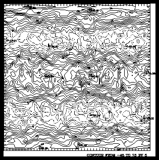
1 CALL CPCNRC (ZREG, M, M, N, -40., 50., 10., 0, 0, -366)
CALL CPCNRC (ZREG, K, M, N, FLOW, FHGH, FINC, NSET, NHGH, NDSH)
CALL SET (.05, .95, .05, .95, WDL, WDR, WDB, WDT, 1)
      CALL GETSET (VPL, VPR, VPB, VPT, ...)
      CALL SET (VPL, VPR, VPB, VPT, WDL, WDR, WDB, WDT, 1)
The first four arguments for CPCNRC are the data array and its dimensions. The fifth and sixth arguments limit the contour lines to be drawn between -40. and 50, and the seventh argument sets the contour interval to 10.
The eighth argument gives NSET the value of zero to produce the default background. The ninth argument sets NHGH to zero, causing highs and lows to be labeled in the style shown.
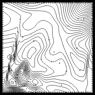
The final argument sets a negative value for NDSH; this plots contour lines with negative values using dashed lines, and it plots contour lines with a zero or a positive value using solid lines. To set NDSH, first create the dash pattern of your choice using a ten-bit binary string where 0 represents a space and 1 represents a dash. The ccpcnrc example started with the number 01011011102; this was then converted to 36610 and used as a negative value for NDSH. This NDSH value specifies the string 01011011100101102 because the first six bits of the 10-bit binary string are copied and added to the end to create a 16-bit string.
Important note: The sequence of calls presented in this Conpack functional outline and shown throughout this Conpack tutorial is commonly used. This approach speeds new users' learning of this sometimes complex material; it does not specify the only way you can use Conpack. As you gain experience using Conpack, you will probably have creative insights that will allow you to achieve a wide variety of results.
This is one of the strengths of Conpack: the order of the calls can be varied to achieve different results in your output plots. When you fill contours with solid colors (called solid fill), you need to draw the background after the fill so the background grid overwrites the fill colors and not vice versa. In other cases, it may be useful to call the background-drawing routine CPBACK before making other drawing calls.
----------------------------------------------------------
 *  1.  Open GKS
    2.  Set window and viewport
    3.  Put in titles and other labels
    4.  Set up general parameters
    5.  Set up area maps
 *  6.  Initialize Conpack
    7.  Force Conpack to choose contour levels if necessary
    8.  Modify Conpack-chosen parameters
    9.  Draw labels
 *  10.  Draw background
 *  11.  Draw contour lines
 *  12.  Call FRAME
 *  13.  Close GKS
----------------------------------------------------------
* Steps needed to produce a contour plot.
For example, Conpack usually uses the dimensions of your data to determine what shape to draw the rectangle around your contours (the contour rectangle). So you can't ask Conpack to draw a perimeter around your contours until it has your data. However, most of us think about drawing the boundary of a plot before drawing contours in it. Therefore, this tutorial first discusses drawing contour rectangles and other backgrounds for Conpack before it discusses Conpack initialization, which is typically the first Conpack call in a program.
The following lines are highlighted in the Conpack functional outline:
Because opening GKS, closing GKS, and clipping are discussed in the NCAR Graphics Fundamentals guide, they are discussed only very briefly here. GKS must be opened and closed for every CGM file---these calls are included in the Conpack functional outline as a reminder that graphics code does not run without them.
Conpack can be initialized with one of the three routines CPRECT, CPSPS1, or CPSPS2, depending on the type of data to be contoured. Section "Cp 3. Initializing Conpack" describes each type of data and the appropriate method for initializing Conpack in each case.
Contour lines are drawn with either a call to CPCLDR or CPCLDM. If you just want to draw contour lines, use CPCLDR. If you want to protect your labels from being drawn over by contour lines, or if you need to use Areas for some other reason, use CPCLDM.
As discussed in the NCAR Graphics Fundamentals guide, FRAME is an SPPS routine that flushes all the buffers and closes a frame so that you can either quit NCAR Graphics or draw another picture. FRAME must be called to finish a Conpack plot, and it is included in the Conpack functional outline as a reminder that you must always call it.
The first argument in a call to CPGETI, CPSETI, CPGETR, CPSETR, CPGETC, or CPSETC is the parameter name. The second argument is either a variable in which the value of the named parameter is to be returned (via CPGETx) or an expression specifying the desired new value of the parameter (via CPSETx).
      CALL CPGETC (PNAM, CVAL)
      CALL CPGETI (PNAM, IVAL)
      CALL CPGETR (PNAM, RVAL)
      CALL CPSETC (PNAM, CVAL)
      CALL CPSETI (PNAM, IVAL)
      CALL CPSETR (PNAM, RVAL)
      CALL CPRSET
The CPRSET subroutine allows you to quickly reset all of the Conpack parameters to their default values between contour plots.
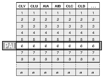
Some of the parameters are not simple integers or reals, but arrays. To access an individual element of a specific parameter array, you can specify individual elements using PAI (Parameter Array Index). For example, to set the ith element of the CLV array, first set PAI=I, then set CLV to the desired value, let's say 0.25:
      CALL CPSETI ('PAI', I)
      CALL CPSETR ('CLV', .25)
These calls set the ith contour level value to 1/4.As individual parameters are described, examples of the CPSETx and CPGETx routines are shown, and the parameters that require CPSETx or CPGETx routine calls are clearly indicated.
Some parameters are described as Fortran type integer, or as integer arrays. These values can be set using:
CALL CPSETI ('PAR', ipar)
or
CALL CPSETR ('PAR', REAL(ipar))
where PAR is some integer parameter and ipar represents its integer value.You can also set a real parameter using:
CALL CPSETI ('XXX', ival)
if the desired value is REAL(ival).Caution: To avoid a common user problem, be sure to double-check your GET and SET calls to ensure that you don't mix integer and real parameters.
Note: The Gridall or Autograph utilities are often used to draw backgrounds for Conpack; these calls can be made before you initialize Conpack.
----------------------------------------------------------
    1.  Open GKS
    2.  Set window and viewport
    3.  Put in titles and other labels
 *  4.  Set up general parameters
    5.  Set up area maps
    6.  Initialize Conpack
    7.  Force Conpack to choose contour levels if necessary
    8.  Modify Conpack-chosen parameters
    9.  Draw labels
 *  10.  Draw background
    11.  Draw contour lines
    12.  Call FRAME
    13.  Close GKS
----------------------------------------------------------
* Steps discussed in this section.
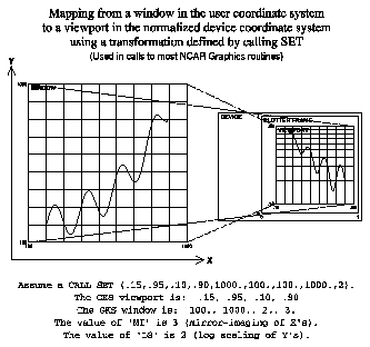
The illustration shows how the coordinate system of your data (the user coordinate system) is mapped first into a window, then into the viewport (a portion of your display screen). Before any graphics can be drawn, the window, viewport, and the transformation between them must be set up so that everything can be drawn correctly.
The best way to set up the window, the viewport, and the transformation in NCAR Graphics is to call the SPPS routine SET. SET sets up the normalization transformation between the user coordinate system and the normalized device coordinate (NDC) system of the viewport. In other words, you call the SPPS routine SET to tell the graphics package the limits of your data space and where on the screen or paper you want your plot to be drawn.
Conpack has 15 different internal parameters that directly affect how Conpack makes a SET call: VPL, VPR, VPB, VPT, VPS, WDL, WDR, WDB, WDT, XC1, XCM, YC1, YCN, SET, and MAP.
The simplest background you can make is to draw a perimeter around your plot using the Conpack routine CPBACK. This does not require you to use any of the above parameters. By default, CPBACK calls the SPPS routine SET for you. This option is covered in module "Cp 2.2 Drawing a contour perimeter."
The next easiest background you can make is to use XC1, XCM, YC1, and YCN to define the X and Y coordinates of your data in the user coordinate system. In this case, you probably want to let Conpack call the SPPS routine SET for you. This option is covered in module "Cp 2.3 Setting X/Y axis values for a contour background."
If you are drawing a map background with Ezmap, you need to follow the Ezmap chapter to set up your map. After the map background is initialized, you can tell Conpack to overlay your data on a map by setting the MAP parameter, then by setting your minimum and maximum latitude and longitude data locations using XC1, XCM, YC1, and YCN. In this case, Ezmap calls the SPPS routine SET for you, so you must tell Conpack that SET has already been called; you do this by setting the Conpack parameter SET. This option is covered in detail in module "Cp 3.8 Non-Cartesian data: Latitude/longitude data."
One of the most complex things that you can do with these options is to use a transformation to map your data to some other place on the plane by setting the Conpack parameter MAP. Then you might set XC1, YC1, XCM, YCN, WDB, WDT, WDL, and WDR to direct the drawing of contours in the window that you define. Setting the window parameters is very similar to setting the viewport parameters; see module "Cp 2.6 Contour perimeter: Size, shape, and location using Conpack."
Occasionally, you may want to use another utility with Conpack, or you may want to call SET yourself. In this case, you simply set the Conpack parameter SET to zero, then make your call to the SPPS routine SET. This option is covered in module "Cp 2.7 Contour perimeter: Size, shape, and location using SET."
In all of the above situations where Conpack calls SET, you can set VPL, VPR, VPB, and VPT to move the plot around on the plotter frame, and you can use VPS to define the desired proportions of your contour plot. Moving your plot around on the plotter frame and changing its proportions is covered in module "Cp 2.6 Contour perimeter: Size, shape, and location using Conpack."

1       CALL CPRECT (Z, K, M, N, RWRK, LRWK, IWRK, LIWK)
2       CALL CPBACK (Z, RWRK, IWRK)
CALL CPBACK (Z, RWRK, IWRK)
Line 1 of the ccpback.f code segment initializes Conpack with a call to CPRECT. This call is thoroughly discussed in module "Cp 3.2 Dense gridded data" and is mentioned here as a reminder that CPBACK must not be called before initializing Conpack. Line 2 calls CPBACK to draw a perimeter around the contours (contours are not drawn in this example).
Perimeter attributes such as line width, line pattern, line color, and so forth can be changed with the same parameters you use with contour lines. Please see the line attributes modules Cp 4.11 through Cp 4.14.
If you have non-Cartesian data, you need to set the MAP parameter to some nonzero value by using the CPSETI routine. Setting the MAP parameter has the side effect of causing CPBACK to do nothing. Hence, if you have non-Cartesian data, and you want a perimeter around your plot, you need to draw it with the GKS routine GPL, the Dashline routine CURVED, the Gridall utility, or the Autograph utility.
      CALL CPSETR ('XC1', XMIN)
      CALL CPSETR ('XCM', XMAX)
      CALL CPSETR ('YC1', YMIN)
      CALL CPSETR ('YCN', YMAX)
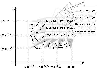
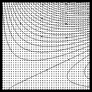
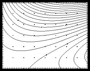
In the default mapping illustration, note that XC1=1.0, XCM=REAL(m), YC1=1.0, and YCN=REAL(n). Also notice how the usual drawing of the Z array is rotated into the Cartesian plane.
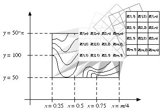
In the user mapping illustration, the user sets XC1=0.25, XCM=m/4.0, YC1=50, and YCN=50*n. In this case, the data are both translated on the X/Y plane and stretched to fit. Any real values for XC1, XCM, YC1, and YCN are allowable, making any translation from a data array to the Cartesian plane possible.
In cases where XC1>XCM, the mapping will be mirror imaged in the X direction.
In cases where YC1>YCN, the mapping will be mirror imaged in the Y direction.
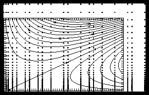
1       CALL CPSETR ('XC1 - X COORDINATE AT INDEX 1', 2.0)
2       CALL CPSETR ('XCM - X COORDINATE AT INDEX M', 20.0)
3       CALL CPSETR ('YC1 - Y COORDINATE AT INDEX 1', 0.0)
4       CALL CPSETR ('YCN - Y COORDINATE AT INDEX N', .01)
5       CALL CPRECT (Z, K, M, N, RWRK, LRWK, IWRK, LIWK)
6       CALL LABMOD ('(E7.2)', '(E7.2)', 0, 0, 10, 10, 0, 0, 1)
7       CALL GRIDAL (K-1, 0, N-1, 0, 1, 1, 5, 0., 0.)
CALL GRIDAL (MJRX, MNRX, MJRY, MNRY,IXLB, IYLB, IGPH, XINT, YINT)
If the axis is linear, MJRX specifies the number of major divisions of the X/Y axis, and MNRX specifies the number of minor divisions within each major division. These values specify the number of spaces between GRIDAL lines or ticks, not the number of lines or ticks. Counting those at the ends, there is always one more major tick than the number of major divisions specified by MJRX. There is always one less minor tick than the number of minor divisions specified by MNRX.
If the axis is logarithmic, major division points occur at a value 10MJRX times the previous point. So if the minimum and maximum X-axis values are 3. and 3000., and MJRX is 1, then the major division points are 3., 30., 300., and 3000. If MNRX<=10, nine minor divisions occur between major divisions. For example, between 3. and 30., there would be minor division points at 6., 9., 12., 15., 18., 21., 24., and 27. If MNRX>10., minor divisions are omitted.
--------------------------
IGPH  X axis     Y axis
--------------------------
0     grid       grid
1     grid       perimeter
2     grid       axis
4     perimeter  grid
5     perimeter  perimeter
6     perimeter  axis
8     axis       grid
9     axis       perimeter
10    axis       axis
--------------------------

1       CALL CPSETR ('XC1 - X COORDINATE AT INDEX 1', 2.0)
2       CALL CPSETR ('XCM - X COORDINATE AT INDEX M', 20.0)
3       CALL CPSETR ('YC1 - Y COORDINATE AT INDEX 1', 0.0)
4       CALL CPSETR ('YCN - Y COORDINATE AT INDEX N', .01)
5       CALL CPRECT (Z, K, M, N, RWRK, LRWK, IWRK, LIWK)
6       CALL LABMOD ('(E7.2)', '(E7.2)', 0, 0, 10, 10, 0, 0, 1)
7       CALL GRIDAL (K-1, 0, N-1, 0, 1, 1, 5, 0., 0.)
CALL LABMOD (FMTX, FMTY, NUMX, NUMY, ISZX, ISZY, IXDC, IYDC, IXOR)
1       CALL CPSETR ('VPL - VIEWPORT LEFT', 0.02)
2       CALL CPSETR ('VPR - VIEWPORT RIGHT', 0.48)
3       CALL CPSETR ('VPB - VIEWPORT BOTTOM', 0.52)
4       CALL CPSETR ('VPT - VIEWPORT TOP', 0.98)
5       CALL CPSETR ('VPL - VIEWPORT LEFT', 0.52)
6       CALL CPSETR ('VPR - VIEWPORT RIGHT', 0.98)
7       CALL CPSETR ('VPB - VIEWPORT BOTTOM', 0.52)
8       CALL CPSETR ('VPT - VIEWPORT TOP', 0.98)
9       CALL CPSETR ('VPS - VIEWPORT SHAPE', -0.33)
10      CALL CPSETR ('VPL - VIEWPORT LEFT', 0.02)
11      CALL CPSETR ('VPR - VIEWPORT RIGHT', 0.48)
12      CALL CPSETR ('VPB - VIEWPORT BOTTOM', 0.02)
13      CALL CPSETR ('VPT - VIEWPORT TOP', 0.48)
14      CALL CPSETR ('VPS - VIEWPORT SHAPE', -1.5)
      CALL CPSETR ('VPL', vpl)
      CALL CPSETR ('VPR', vpr)
      CALL CPSETR ('VPB', vpb)
      CALL CPSETR ('VPT', vpt)
      CALL CPSETR ('VPS', vps)
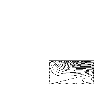
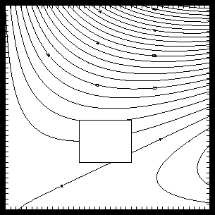
In the ccpvp.f program, there are calls to Conpack routines that draw contours between lines 4 and 5, lines 9 and 10, and lines 14 and 15 of the code segment. Lines 1 through 4 of the ccpvp.f code segment set up the viewport so that the first plot is drawn in the upper left corner. Lines 5 through 8 put the second plot in the upper right corner. Line 9 specifies a contour rectangle three times as high as it is wide.
Lines 10 through 13 tell Conpack to draw contours in the lower left corner, and line 14 specifies a contour rectangle wider than it is tall. This contour drawing uses rho/theta data; this is why it draws contours in a wedge rather than a square.
Contours in the lower right corner are drawn without setting VPR, VPL, VPB, or VPT because the viewport is set up by Ezmap.
1       CALL SET (0.5, 0.98, 0.125, 0.375, 0., 2., 0., 1., 1)
2       CALL CPSETI ('SET - DO-SET-CALL FLAG', 0)
3       CALL CPSETR ('XC1 - X COORDINATE AT INDEX 1', 0.)
4       CALL CPSETR ('XCM - X COORDINATE AT INDEX M', 2.)
5       CALL CPSETR ('YC1 - Y COORDINATE AT INDEX 1', 0.)
6       CALL CPSETR ('YCN - Y COORDINATE AT INDEX N', 1.)
7       CALL CPRECT (Z, K, M, N, RWRK, LRWK, IWRK, LIWK)
8       CALL CPBACK (Z, RWRK, IWRK)
9       CALL CPCLDR (Z, RWRK, IWRK)
      CALL CPSETI ('SET', iset)
      CALL SET (VL, VR, VB, VT, WL, WR, WB, WT, LS)
The call to SET in line 1 of the ccpset.f code segment defines the portion of the plotter frame used for the plot. Line 2 uses the Conpack parameter SET to tell Conpack that subroutine SET has already been called. Lines 3 through 6 place the contour rectangle in the X/Y plane. XC1, XCM, YC1, and YCN are the same as WL, WR, WB, and WT in the SET call because this is where user coordinates are defined for Conpack and SET. Contours are then initialized and drawn normally. Because CPRECT, CPSPS1, and CPSPS2 all use information specified in the CPSETx calls, it is best to set general parameters before calling the Conpack initialization routines.
CALL CPSETI ('SET', 0)
and explain the results.
----------------------------------------------------------
    1.  Open GKS
    2.  Set window and viewport
    3.  Put in titles and other labels
    4.  Set up general parameters
    5.  Set up area maps
 *  6.  Initialize Conpack
    7.  Force Conpack to choose contour levels if necessary
    8.  Modify Conpack-chosen parameters
    9.  Draw labels
    10.  Draw background
    11.  Draw contour lines
    12.  Call FRAME
    13.  Close GKS
----------------------------------------------------------
* Steps discussed in this section.
Dense gridded data  Sparse gridded data

Irregularly spaced gridded data  Missing data

Nongridded data

Non-Cartesian data  Non-Cartesian data

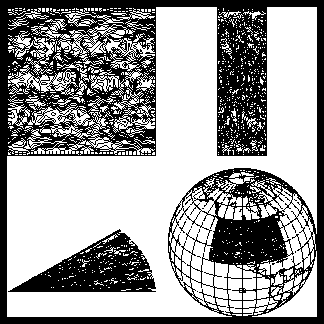
Generally, if your data set has less than 35 data points in either direction, it is better to use CPSPS1. However, this distinction is very subjective. Most modelers define "sparse" for global datasets as a spacing of 2 degrees or more between data points.
Bivar, an interpolation package that works with Conpack, is distributed with NCAR Graphics. Bivar can be used on data that do not have abrupt changes (like ridges or cliffs on a topographic map). In other words, Bivar assumes that the function describing the data has a continuous first derivative. If your data do not fit this description, or if you have an interpolation package that fits your data better, don't use Bivar.
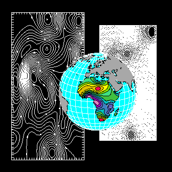
Latitude/longitude data is fairly common, and Conpack is designed so that it is easy to overlay lat/lon data over a map.
Conpack can also easily be used to display polar coordinate data, using a method similar to the lat/lon display method.
Almost any data that can be transformed into data on a rectangular grid can be contoured by Conpack by writing a transformation, and adding it to the CPMPXY subroutine provided by Conpack.
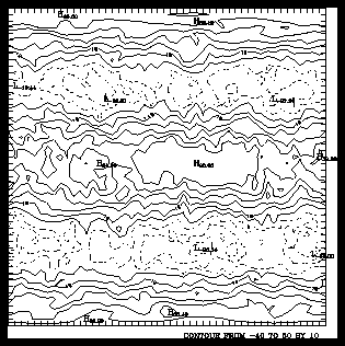
1       CALL CPRECT (Z, M, M, N, RWRK, LRWK, IWRK, LIWK)
2       CALL CPBACK (Z, RWRK, IWRK)
3       CALL CPCLDR (Z, RWRK, IWRK)
4       CALL MARK (M, N)
CALL CPRECT (Z, K, M, N, RWRK, LRWK, IWRK, LIWK)
Occasionally you may see error messages similar to this:
CPGRWS     200 WORDS REQUESTED, 100
WORDS AVAILABLE
CPGIWS     200 WORDS REQUESTED, 100
WORDS AVAILABLE
CPGRWS tells you that your real workspace is too small, and CPGIWS tells you that your integer workspace is too small. Increase LRWK or LIWK to the number of words requested in the error message, and repeat until the error message goes away.
The size of LRWK and LIWK depends on the complexity of your contour plot, so plots with lots of small, tight contour levels require more space than large, loose contour plots like ccprect. If you are running a job with lots of similar plots, and need to minimize workspace, see module "Cp 3.12 Setting minimal workspace" for the most reliable method of optimizing these array sizes.
      Z(I,J) = sin(1./real(i*j)) * sin(real(i*j)) *


      cos(real(i)/real(j)) + cos(real(i*j))
in subroutine GETDAT instead.
1       CALL CPSPS1 (Z, K, M, N, RWRK, LRWK, IWRK, LIWK, ZDAT, LZDT)
2       CALL CPBACK (ZDAT, RWRK, IWRK)
3       CALL CPCLDR (ZDAT, RWRK, IWRK)
4       CALL MARK (X, Y, M, N)
CALL CPSPS1 (ZSPS, K, M, N, RWRK, LRWK, IWRK, LIWK, ZREG, LZRG)
100 * ((NSPV+99)/100) + 3 * M * N + MAX (M + N + N, 4 * IZDM)
100 * ((NSPV+99)/100)
If your sparse array defines a long, narrow rectangle, Conpack chooses a roughly square rectangle of contours for you. It is possible to change this by specifying the dimensions of the interpolated array ZREG, using the parameters ZDS, ZDM, and ZDN. For more information on changing the shape of your contour rectangle, see the contour perimeter modules Cp 2.6 and Cp 2.7.
By default, both CPSPS1 and CPSPS2 use bicubic splines under tension to fit the sparse array data values. The routines used are from Fitpack, by Alan Cline. Spline tension can be changed with the T2D parameter. More information appears in module "Cp 9.1 Smoothing contours."
Occasionally you may see error messages like this:
CPGRWS     200 WORDS REQUESTED, 100
WORDS AVAILABLE
CPGIWS     200 WORDS REQUESTED, 100
WORDS AVAILABLE
CPGRWS tells you that your real workspace is too small, and CPGIWS tells you that your integer workspace is too small. Increase LRWK or LIWK to the number of words requested in the error message, and repeat until the error message goes away.
CPSPS1 cannot extrapolate data beyond the boundaries of the data field.
1       CALL CPSPS2 (X, Y, Z, M, M, N, RWRK, LRWK, IWRK, LIWK, ZREG, LZRG)
2       CALL CPBACK (ZREG, RWRK, IWRK)
3       CALL CPCLDR (ZREG, RWRK, IWRK)
4       CALL MARK (X, Y, M, N)
CALL CPSPS2 (X, Y, Z, K, M, N, RWRK, LRWK, IWRK, LIWK, ZREG, LZRG)
LRWK \xb3 100 * ((NSPV+99)/100) + 3 * M * N + M + N + N)
LIWK >= 100 * ((NSPV+99) / 100)
LZRG = MAX (1600, M * N)
If your sparse array defines a long, narrow rectangle, Conpack chooses a roughly square rectangle of contours for you. It is possible to change this by specifying the dimensions of the interpolated array ZREG, using the parameters ZDS, ZDM, and ZDN. For more information on changing the shape of your contour rectangle, see the contour perimeter modules Cp 2.6 and Cp 2.7.
By default, both CPSPS1 and CPSPS2 use bicubic splines under tension to fit the sparse array data values. The routines used are from Fitpack, by Alan Cline. Spline tension can be changed with the T2D parameter. More information appears in module "Cp 9.1 Smoothing contours."
Occasionally you may see error messages similar to this:
CPGRWS     200 WORDS REQUESTED, 100
WORDS AVAILABLE
CPGIWS     200 WORDS REQUESTED, 100
WORDS AVAILABLE
CPGRWS tells you that your real workspace is too small, and CPGIWS tells you that your integer workspace is too small. Increase LRWK or LIWK to the number of words requested in the error message, and repeat until the error message goes away.
CPSPS2 cannot extrapolate data beyond the boundaries of the data field.
Another common error is the failure to specify the arrays X and Y in strictly increasing order. When this happens, you see this error message:
ERROR 6 IN CPSPS2 - ERROR IN CALL TO MSSRF1
1       DO 101, I=2, MREG
2          XREG(I) = XMIN + (XMAX-XMIN) * REAL(I-1)/(MREG-1)
3  101  CONTINUE
4       DO 102, I=2, NREG
5          YREG(I) = YMIN + (YMAX-YMIN) * REAL(I-1)/(NREG-1)
6  102  CONTINUE
7       CALL IDSFFT (1, NRAN, XRAN, YRAN, ZRAN, MREG, NREG, MREG, XREG, YREG,
       + ZREG, IWRK, RWRK)
8       CALL CPRECT (ZREG, MREG, MREG, NREG, RWRK, LRWK, IWRK, LIWK)
9       CALL CPCLDR (ZREG, RWRK, IWRK)
10      CALL MARK (XRAN, YRAN, NRAN)
      CALL IDSFFT (MD, NRAN, XRAN, YRAN, ZRAN, MREG, NREG, KREG, XREG,
     +             YREG, ZREG, IWK, WK)
Bivar requires that nongridded data points must be distinct and their projections in the X/Y plane must not be collinear. In other words, you can't have two Z values for the same X,Y pair, and your X,Y values can't all lie on the same line.
Inadequate work space in IWK and WK may cause incorrect results. If you decide to share the work arrays with Conpack work arrays, make sure that your integer work space is large enough. In general, IDSFFT needs more integer space than Conpack, and Conpack needs more real work space than IDSFFT. Also, Conpack relies on the fact that workspace arrays are not modified between calls to Conpack routines, so IDSFFT must be called before calls to Conpack.
In versions of NCAR Graphics prior to Version 3.2, you must load your own copy of Bivar for use with nongridded data. First, execute:
C PACKAGE BIVARThe remainder of the file is the Bivar package. In NCAR Graphics Version 3.2, Bivar resides in libncarg.a, so you only need to load the NCAR Graphics library to use Bivar.
1       CALL CPSETR ('SPV - SPECIAL VALUE', -1.0)
2       CALL CPSETI ('PAI - PARAMETER ARRAY INDEX', -2)
3       CALL CPSETI ('CLU - CONTOUR LEVEL USE FLAGS', 1)
4       CALL CPRECT (Z, K, M, N, RWRK, LRWK, IWRK, LIWK)
5       CALL CPBACK (Z, RWRK, IWRK)
6       CALL CPCLDR (Z, RWRK, IWRK)
      CALL CPSETR ('SPV', spv)
      CALL CPSETI ('PAI', ipai)
      CALL CPSETI ('CLU', iclu)
Non-Cartesian data Non-Cartesian data

Then decide what kind of data you have in the Cartesian space (for example dense gridded, sparse gridded, irregularly spaced gridded, or nongridded), and initialize for that type of data. After these steps are done, contours are drawn normally. The next few modules discuss examples of how to use your data in various non-Cartesian spaces.
      CPSETI ('MAP', 1)
      CPSETR ('XC1', xmin)
      CPSETR ('XCM', xmax)
      CPSETR ('YC1', ymin)
      CPSETR ('YCN', ymax)
      CPSETR ('ORV', val)
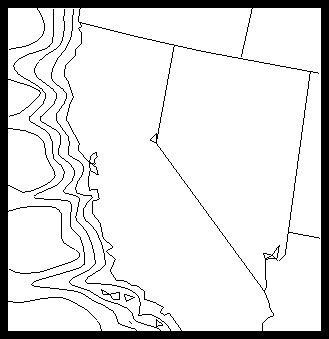
1       PARAMETER (RMNLON=-190., RMXLON=20., RMNLAT=-20., RMXLAT=50.)
2       DATA RLAT1 /RMNLAT, 0.0/
3       DATA RLAT2 /RMXLAT, 0.0/
4       DATA RLON1 /RMNLON, 0.0/
5       DATA RLON2 /RMXLON, 0.0/
6       CALL MAPSTI ('GR - GRID', 10)
7       CALL MAPSTC ('OU - OUTLINE DATASET', 'PO')
8       CALL MAPROJ ('SV - SATELLITE-VIEW', 35., -100., 0.)
9       CALL MAPSET ('MA', RLAT1, RLON1, RLAT2, RLON2)
10      CALL MAPDRW
11      CALL CPSETI ('SET - DO-SET-CALL FLAG', 0)
12      CALL CPSETR ('XC1 - X COORDINATE AT INDEX 1', RMNLON)
13      CALL CPSETR ('XCM - X COORDINATE AT INDEX M', RMXLON)
14      CALL CPSETR ('YC1 - Y COORDINATE AT INDEX 1', RMNLAT)
15      CALL CPSETR ('YCN - Y COORDINATE AT INDEX N', RMXLAT)
16      CALL CPSETI ('MAP - MAPPING FLAG', 1)
17      CALL CPSETR ('ORV - OUT-OF-RANGE VALUE', 1.E12)
18      CALL CPRECT (Z, M, M, N, RWRK, LRWK, IWRK, LIWK)
19      CALL CPCLDR (ZREG, RWRK, IWRK)
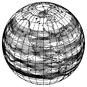
Lines 1 through 5 of the ccpmap.f code segment set the minimum and maximum latitude and longitude values for both the geographic and contour mappings. Lines 6 through 10 draw a black-and-white map of the globe using routines discussed in the Ezmap chapter. Line 6 specifies that latitude and longitude lines should be drawn at 10-degree intervals. Line 7 forces drawing of political and continental boundary lines. Lines 8 and 9 specify a satellite view of the globe. Line 10 draws the map. Up to this point, everything is just as it would be if no contours were to be drawn.
Lines 11 through 19 overlay contours on the Ezmap projection. As discussed in module "Cp 2.7 Contour perimeter: Size, shape, and location using SET," the Conpack parameter SET in line 11 tells Conpack that subroutine SET has been called by Ezmap. XC1, XCM, YC1, and YCN fix the corners of the array on the globe. Line 16 sets the Conpack parameter MAP so that Conpack knows that lat/lon data is being used. Line 12 sets ORV to "1.E12" so that contours will be terminated at the edge of the visible portion of the globe. Notice that all of the parameter-setting routines are called before the CPRECT call to initialize Conpack for drawing.
Lines 18 and 19 initialize Conpack and draw contours in the same way as for a simple Cartesian plot.
In some cases, you may want to draw contours across the international date line. To do this, you must make sure that XC1<XCN, even if it means making XCN>180. Notice that contours are drawn across the date line in the example.
1       CALL SET (0.05, 0.95, 0.05, 0.95, -RHOMX, RHOMX, -RHOMX, RHOMX, 1)
2       CALL CPSETI ('SET - DO-SET-CALL FLAG', 0)
3       CALL CPSETR ('XC1 - X COORDINATE AT INDEX 1', RHOMN)
4       CALL CPSETR ('XCM - X COORDINATE AT INDEX M', RHOMX)
5       CALL CPSETR ('YC1 - Y COORDINATE AT INDEX 1', THETMN)
6       CALL CPSETR ('YCN - Y COORDINATE AT INDEX N', THETMX)
7       CALL CPSETI ('MAP - MAPPING FLAG', 2)
8       CALL CPRECT (Z, M, M, N, RWRK, LRWK, IWRK, LIWK)
9       CALL CPCLDR (ZREG, RWRK, IWRK)
      CPSETR ('XC1', rho-min)
      CPSETR ('XCM', rho-max)
      CPSETR ('YC1', theta-min)
      CPSETR ('YCN', theta-max)
      CPSETI ('MAP', imap)
Line 7 sets the MAP parameter so that Conpack knows we are using polar coordinates. Notice that all of the parameters are set before the CPSPS2 call to initialize Conpack for drawing.
Lines 8 and 9 initialize Conpack and draw contours just as they would be for a simple Cartesian plot.
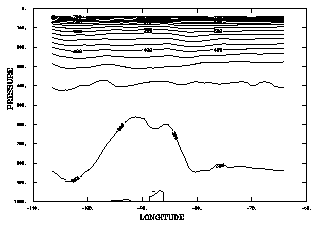
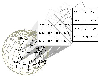
1       SUBROUTINE CPMPXY (IMAP, XINP, YINP, XOTP, YOTP)
2       PARAMETER (JX=60, KX=26)
3       COMMON /HEIGHT/ Z (JX, KX)
4       ELSEIF (IMAP .EQ. 3 .OR. IMAP .EQ. 4) THEN
5         XOTP = XINP
6         X = XINP
7         IIX = INT(X)
8         DIFX = X - FLOAT(IIX)
9         Y = YINP
10        IY = INT(Y)
11        DIFY = Y - FLOAT(IY)
12        IXP1 = MIN0 (JX, IIX + 1)
13        IYP1 = MIN0 (KX, IY + 1)
14        Z1 = Z(IIX, IY) + DIFY * (Z(IIX, IYP1) - Z(IIX, IY))
15        Z2 = Z(IXP1, IY) + DIFY * (Z(IXP1, IYP1) - Z(IXP1, IY))
16        ZR = Z1 + DIFX * (Z2 - Z1)
17        YOTP = ZR
18        IF (IMAP .EQ. 4) YOTP = 1000. * EXP (-ZR / 7.)
SUBROUTINE CPMPXY (IMAP, XINP, YINP, XOTP, YOTP)
Line 3 of the ccpmpxy.f code segment passes the data array containing height values into CPMPXY for use in calculating the pressure transformation. Line 4 checks to see whether a height or pressure transformation is specified. Since there is no transformation in the X direction, line 5 gives the X output coordinate the same value as the X input coordinate.
Because the point on the contour line probably is not on one of the grid points in the original data, it is necessary to interpolate the height and pressure data value in this case. Therefore, lines 7 through 15 find the nearest data points in the Y direction and interpolate for the height at the point on the contour line. Line 16 calculates the interpolated height, and line 17 returns it as the Y output coordinate. If the MAP parameter IMAP specifies a pressure transformation, line 18 calculates that transformation and returns the pressure value as the Y output coordinate.
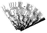
Some contours cannot be allowed to flow over the boundary. For example, ocean temperature doesn't exist over land, so contours showing ocean temperature must follow the shoreline. Unfortunately, the data are usually not dense enough along the boundary to force contours to conform to the boundary line, and worse, Bivar assumes that the data have a continuous first derivative. What this means in practice is that by using the methods discussed in section "Cp 3. Initializing Conpack," contour lines are almost guaranteed to cross boundary lines. When interpolation is being used in cases like this, it may be possible to find an interpolation package that better fits your needs for interpolation libraries (FITPACK may be a good choice).
The amount of workspace needed to produce a contour plot often depends on how many tightly curved contour lines you have and on how several parameters are set. A plot having only a few contours with large, gradual curves needs much less workspace than a plot with small, winding contours.
Although it is possible to calculate an upper bound for both integer and real work arrays, the process is tedious, and it must be done for each Conpack routine called. Please see the Conpack programmer document if you need to calculate an upper bound for your work arrays. It is much easier to let Conpack tell you how much space it needs, and then adjust your array sizes downward to match.
Integer Workspace Used: 100 Real Workspace Used: 200
1       CALL CPRECT (Z, K, M, N, RWRK, LRWK, IWRK, LIWK)
2       CALL CPBACK (Z, RWRK, IWRK)
3       CALL CPCLDR (Z, RWRK, IWRK)
4       CALL CPGETI ('IWU - INTEGER WORKSPACE USAGE', IIWU)
5       CALL CPGETI ('RWU - REAL WORKSPACE USAGE', IRWU)
6       WRITE (6,*) 'Integer Workspace Used: ',IIWU,
       + ' Real Workspace Used: ',IRWU
      CALL CPGETI ('IWU', iwu)
      CALL CPGETI ('RWU', irwu)
Since you use IWU and RWU most frequently when you are planning to run the same job over and over with different data, we recommend that you always make LRWK and LIWK somewhat larger than the values returned by RWU and IWU.
Previous Chapter Tutorial Home Next Chapter